Change of variables of a random variable

Question

I'm looking for a way to perform the change of variable of a random variable. In particular, I've a random variable $X$ with probability density function:

$$ f_X(x) = \begin{cases} a \, e^X \quad &\text{if } x \leq 1 \\ 3 \, (1 - a \, e) \, x^{-4} \quad &\text{if } x > 1 \end{cases} $$

where $a \in [0, \, e^{-1}]$. The goal is to get the probability density function of $Y = X^3$. How can I do it in Mathematica?

The result should be:

---

EDIT: error in $0 < y < 1$: the exponent sign of the exponential $e$ is + not -.

Answer 1

Define the probability distribution for $X$:

fx[a_, x_] = Piecewise[{{a E^x, x <= 1}}, 3 (1 - a E) x^-4];
px[a_] = ProbabilityDistribution[fx[a, x], {x, -∞, ∞}];

Find the PDF of $Y=X^3$:

py[a_] = TransformedDistribution[x^3, Distributed[x, px[a]]];
fy[a_, y_] = PDF[py[a], y]

$$ \begin{cases} \frac{1-e a}{y^2} & y>1 \\ \frac{a e^{\text{Root}\left[\text{$\#$1}^3-y\&,1\right]}}{3 \text{Root}\left[\text{$\#$1}^3-y\&,1\right]^2} & y<1 \\ \text{Indeterminate} & \text{True} \end{cases} $$

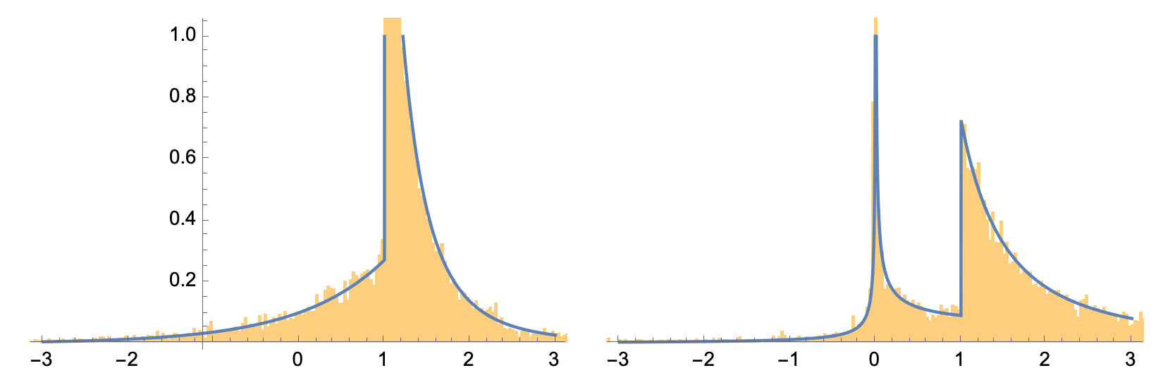
Check numerically for a specific value, for example $a=0.1$:

With[{a = 0.1},
  X = RandomVariate[px[a], 10^4];
  Y = X^3;
  GraphicsRow@{
    Show[
      Histogram[X, {1/30}, "PDF"],
      Plot[fx[a, x], {x, -3, 3}, PlotRange -> {0, 1}], 
      PlotRange -> {{-3, 3}, {0, 1}}], 
    Show[
      Histogram[Y, {1/30}, "PDF"], 
      Plot[fy[a, y], {y, -3, 3}, PlotRange -> {0, 1}], 
      PlotRange -> {{-3, 3}, {0, 1}}]}]

Answer 2

This is just an extended comment based on @Roman's answer.

That answer using Root objects takes care of the cases where $y<0$ and $0<y<1$ just with the restriction $y<1$. But if you want to have the cases where $y<0$ and $0<y<1$ made explicit and have the function look in a more standard way, then you'll need to do some of the work "by hand" using the ToRadicals function.

pdfyLessThan0 = FullSimplify[(a E^Root[-y + #1^3 &, 1])/(3 Root[-y + #1^3 &, 1]^2) //
  ToRadicals, Assumptions -> y < 0]

pdfyBetween0and1 = FullSimplify[(a E^Root[-y + #1^3 &, 1])/(3 Root[-y + #1^3 &, 1]^2), 
  Assumptions -> 0 < y < 1]

pdfyGreaterThan1 = FullSimplify[fy[a, y], Assumptions -> y > 1]

pdfy = Piecewise[{{pdfyLessThan0, y < 0}, {pdfyBetween0and1, 0 < y < 1},
  {pdfyGreaterThan1, y > 1}}, Indeterminate]

And, of course, you need the restriction that $0<a\leq \frac{1}{e}$.

Answer 3

THIS IS AN EXTENDED COMMENT

Clear["Global`*"]

distx3[a_] = ProbabilityDistribution[
   Piecewise[{{a E^x, x <= 1}}, 3 (1 - a E) x^-4], {x, -∞, ∞}];

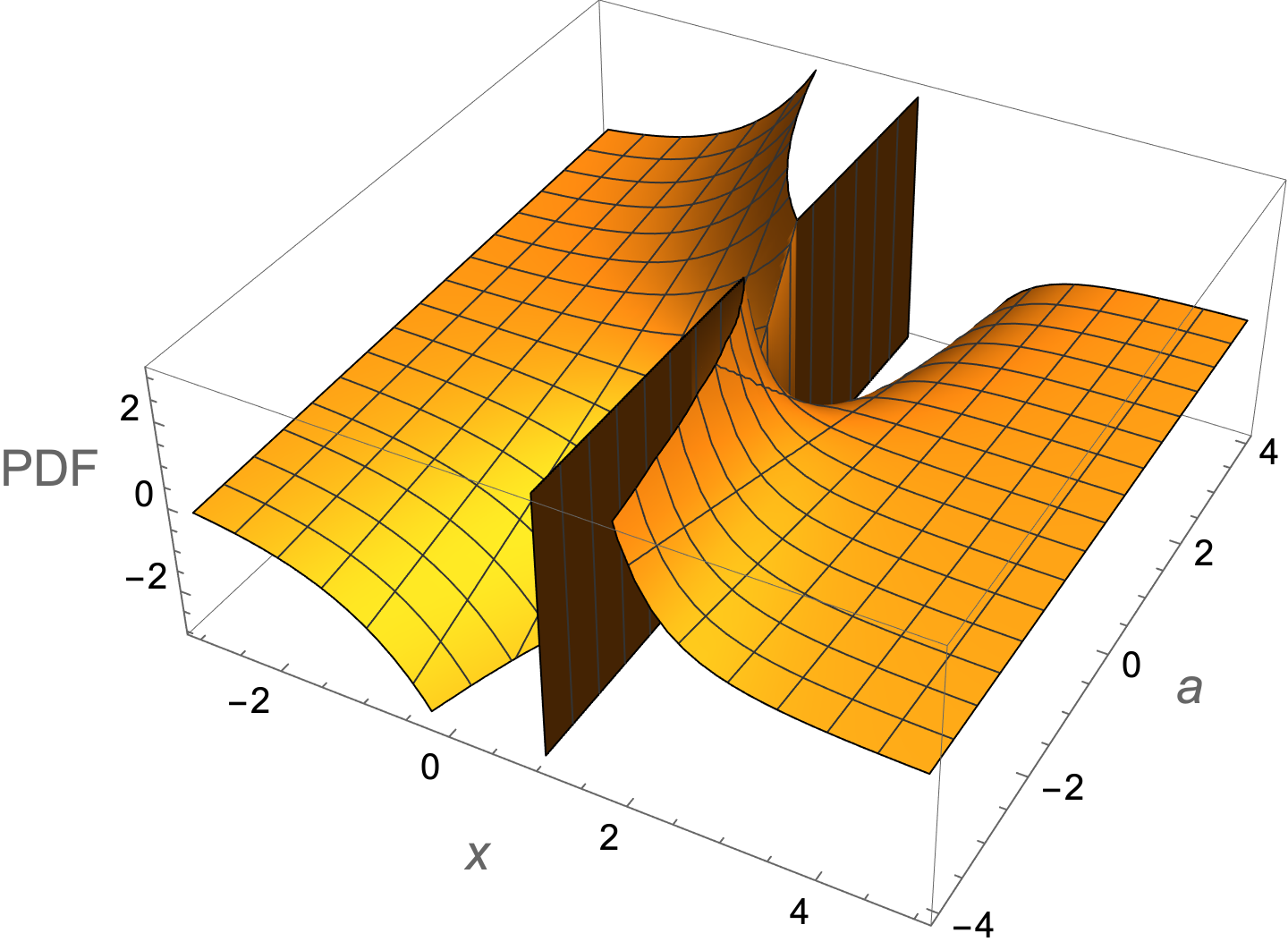
Plotting the PDF of the this distribution

Plot3D[PDF[distx3[a], x],
 {x, -3, 5}, {a, -4, 4},
 PlotPoints -> 50,
 MaxRecursion -> 3,
 ClippingStyle -> None,
 AxesLabel -> (Style[#, 14] & /@ {x, a, PDF})]

Since a PDF cannot be negative, the distribution must be redefined to exclude the regions where the function is negative.

distx2[a_] = ProbabilityDistribution[
   Piecewise[{{a E^x, x <= 1 && a > 0},
     {3 (1 - a E) x^-4, x > 1 && a < 0}}], {x, -∞, ∞}];

However, this is not normalized:

Assuming[a > 0,
 Integrate[PDF[distx2[a] // Simplify, x], {x, -Infinity, Infinity}]]

(* a E *)

Assuming[a < 0,
 Integrate[PDF[distx2[a] // Simplify, x], {x, -Infinity, Infinity}]]

(* 1 - a E *)

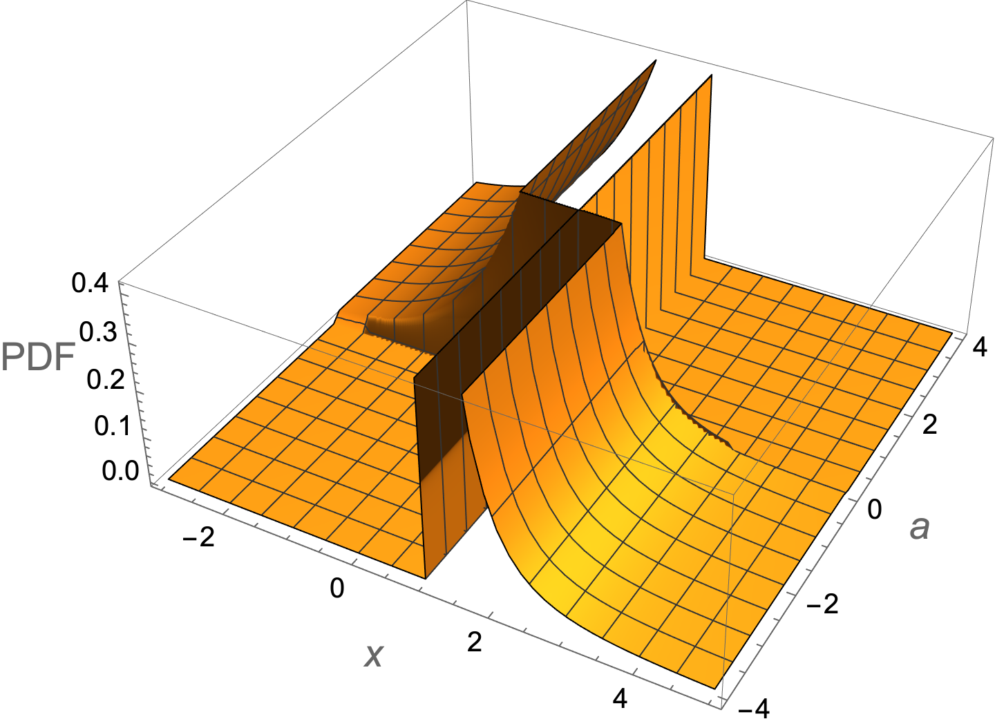
Normalizing the distribution gives

distx[a_] = ProbabilityDistribution[
   Piecewise[{{E^(x - 1), x <= 1 && a > 0},
     {3 x^-4, x > 1 && a < 0}}], {x, -∞, ∞}];

Plot3D[PDF[distx[a], x],
 {x, -3, 5}, {a, -4, 4},
 PlotPoints -> 50,
 MaxRecursion -> 3,
 ClippingStyle -> None,
 AxesLabel -> (Style[#, 14] & /@ {x, a, PDF})]

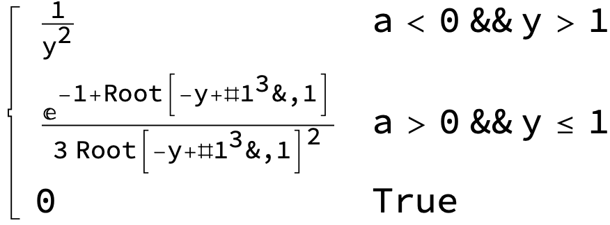
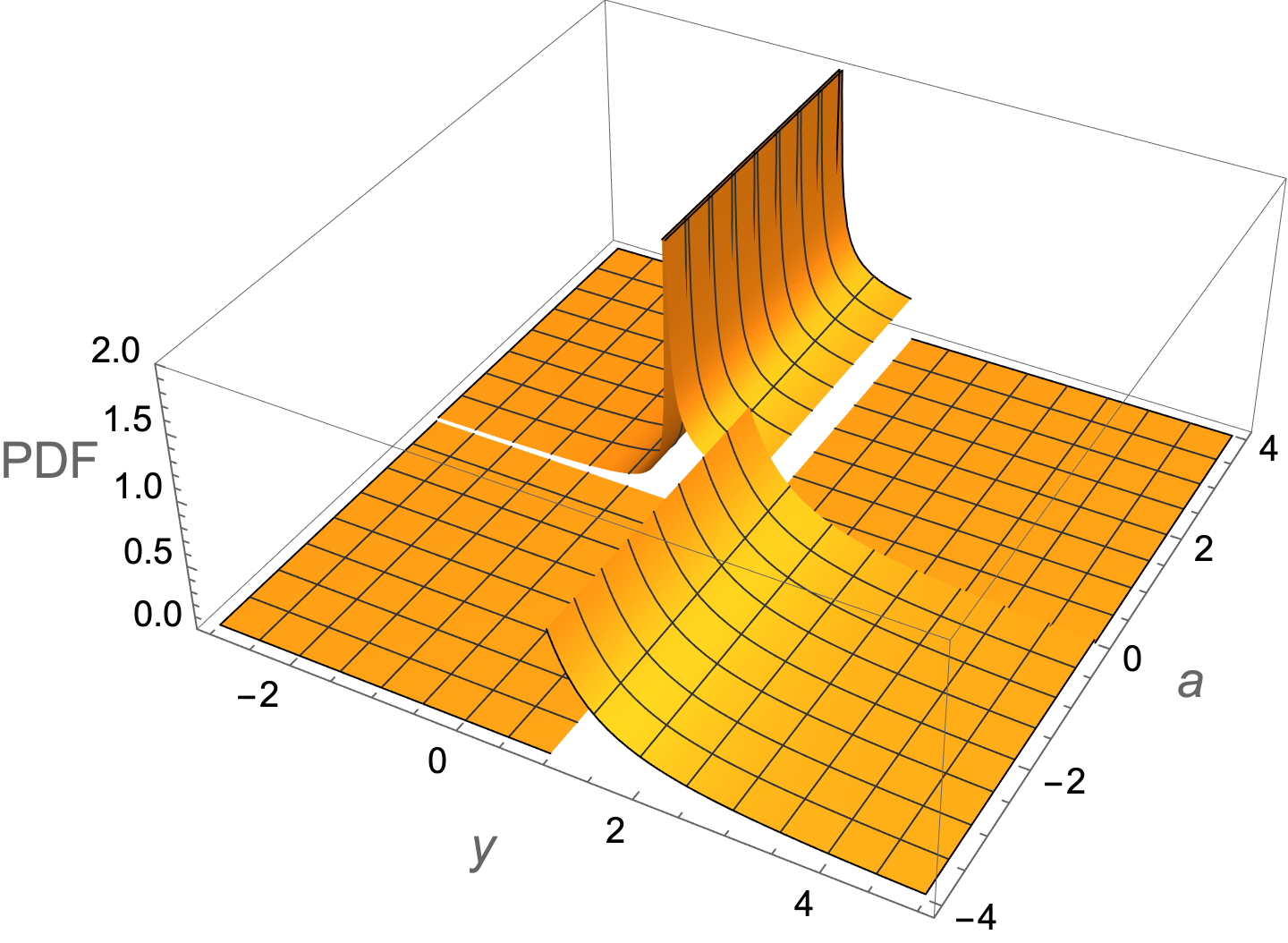
disty[a_] = TransformedDistribution[x^3, Distributed[x, distx[a]]];

PDF[disty[a], y]

Plot3D[Evaluate@PDF[disty[a], y],
 {y, -3, 5}, {a, -4, 4},
 PlotRange -> {0, 2},
 PlotPoints -> 75,
 MaxRecursion -> 4,
 ClippingStyle -> None,
 AxesLabel -> (Style[#, 14] & /@ {y, a, PDF})]