In the 90s, several turbulence models were proposed. Using Mathematica vv 10-12.1 we tested two models:
Spalart-Allmaras turbulence model (SA) for aerodynamic applications, published in AIAA Paper 92 - 0439, 1992, see also wikipedia
turbulence model for a nonisothermal atmospheric boundary layer with roughness, buoyancy and flow rotation (TT), published on https://www.witpress.com/Secure/elibrary/papers/AIR96/AIR96028FU.pdf https://www.witpress.com/Secure/elibrary/papers/AIR97/AIR97011FU.pdf
Test. In 2D, at the initial moment of time, a linear velocity profile is set. Define a profile at a later time. Model SA depends on 10 parameters:
sigma = 2/3; kap = .41; cb1 = .1355; cb2 = .622; eps = 10^-6; d =
 Sqrt[y^2 + eps^2]; cw1 =
 cb1/kap^2 + (1 + cb2)/
   sigma; cw2 = .3; cw3 = 2; cv1 = 7.1; ct1 = 1; ct2 = 2; ct3 = 1.2; \
ct4 = .5; mu = 1.711 10^-5;

om = Sqrt[ (D[u[t, x, y], y] - D[u[t, x, y], x])^2];
S = om + (1 - (nu[t, x, y]/
         mu)/(1 + (nu[t, x, y]/
             mu)^4/(cv1^3 + (nu[t, x, y]/mu)^3))) nu[t, x,
      y]/(kap d)^2;
r = nu[t, x, y]/S/(kap d)^2;
fw = (r +
     cw2 (r^6 - r)) ((1 + cw3^6/(cw3^6 + (r + cw2 (r^6 - r))^6)))^(1/
      6);
ft2 = ct3 Exp[-ct4 (nu[t, x, y]/mu)^2];
nut = nu[t, x, y] (nu[t, x, y]/mu)^3/(cv1^3 + (nu[t, x, y]/mu)^3);
(*d=y for the wall*)

L = 10^4; t0 = 15; px = 0;

eq = {D[nu[t, x, y], t] +
     u[t, x, y] D[nu[t, x, y], x] == (cb1 (1 - ft2) S  nu[t, x, y] +
       1/sigma (D[(nut + mu) D[nu[t, x, y], y], y] +
          D[(nut + mu) D[nu[t, x, y], x], x] +
          cb2 (D[nu[t, x, y], x]^2 + D[nu[t, x, y], y]^2)) - (cw1 fw -
           cb1/kap^2 ft2) (nu[t, x, y]/d)^2 )/mu,
   D[u[t, x, y], t] + u[t, x, y] D[u[t, x, y], x] + px ==
    D[(nut/mu + 1) D[u[t, x, y], y], y] + D[u[t, x, y], x, x]};
bc = {nu[t, x, 0] == 0, u[t, x, 0] == 0, u[t, x, L] == 1,
   nu[t, x, L] == 0.1, nu[t, 0, y] == 0.1 y/L, u[t, 0, y] == y/L};
ic = {nu[0, x, y] == 0.1 y/L, u[0, x, y] == y/L};
{nU, U} =
  NDSolveValue[{eq, ic, bc}, {nu, u}, {t, 0, t0}, {x, 0, L}, {y, 0,
    L}];
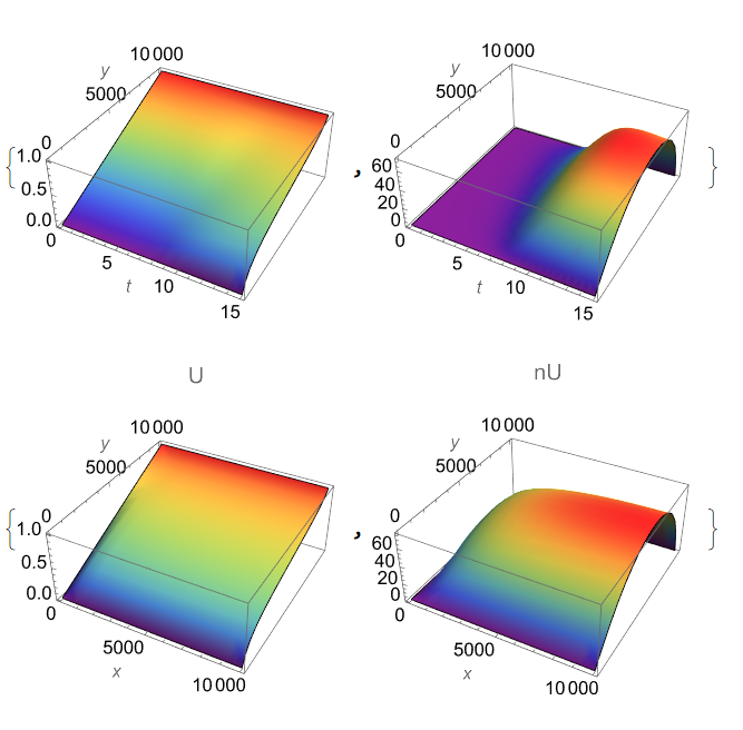
Visualisation
{Plot3D[U[t, L/2, y], {t, 0, t0}, {y, 0, L}, Mesh -> None,
  ColorFunction -> "Rainbow", AxesLabel -> Automatic],
 Plot3D[nU[t, L/2, y], {t, 0, t0}, {y, 0, L}, Mesh -> None,
  ColorFunction -> "Rainbow", AxesLabel -> Automatic]}

{Plot3D[U[t0, x, y], {x, 0, L}, {y, 0, L}, PlotRange -> All,
  AxesLabel -> {x, y, ""}, PlotLabel -> "U", Mesh -> None,
  ColorFunction -> "Rainbow"],
 Plot3D[nU[t0, x, y], {x, 0, L}, {y, 0, L}, PlotRange -> All,
  AxesLabel -> {x, y, ""}, PlotLabel -> "nU", Mesh -> None,
  ColorFunction -> "Rainbow"]}
 Model TT depends on 2 parameters:
T = 3; L = 1000; W0 = .00002; U0 = 1; R = 13.22; px = 0.13; b = \
.0001; eq = {D[W[x, y, t], t] + u[x, y, t] D[W[x, y, t], x] +
    Integrate[W[x, y, t], {y, 0, y}]*D[W[x, y, t], y] -
    2*R*y*D[W[x, y, t], y] - R*(1 + y^2)*D[W[x, y, t], y, y] -
    D[W[x, y, t], x, x] == (y/(1 + y^2))*
     Integrate[W[x, y, t], {y, 0, y}] + b*y/(1 + y^2),
  D[u[x, y, t], t] + u[x, y, t] D[u[x, y, t], x] +
    Integrate[W[x, y, t], {y, 0, y}]*D[u[x, y, t], y] -
    R*y*D[u[x, y, t], y] - R*(1 + y^2)*D[u[x, y, t], y, y] -
    D[u[x, y, t], x, x] + px == 0};
ic = {W[x, y, 0] == W0*(y - L),
  u[x, y, 0] == U0*y/L}; bc = {W[x, L, t] == 0, W[x, 0, t] == -W0*L,
  W[0, y, t] == W0*(y - L), u[x, 0, t] == 0, u[x, L, t] == U0,
  u[0, y, t] == U0*y/L}; bc1 = {Derivative[1, 0, 0][u][L, y, t] == 0,
  Derivative[1, 0, 0][W][L, y, t] == 0};
sol = NDSolve[{eq, ic, bc}, {W, u}, {x, 0, L}, {y, 0, L}, {t, 0, T},
   Method -> {"MethodOfLines",
     "SpatialDiscretization" -> {"TensorProductGrid",
       "MinPoints" -> 150}}];
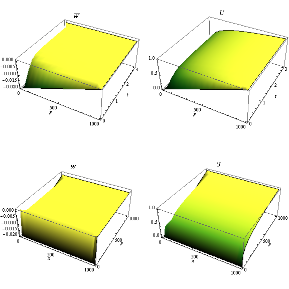
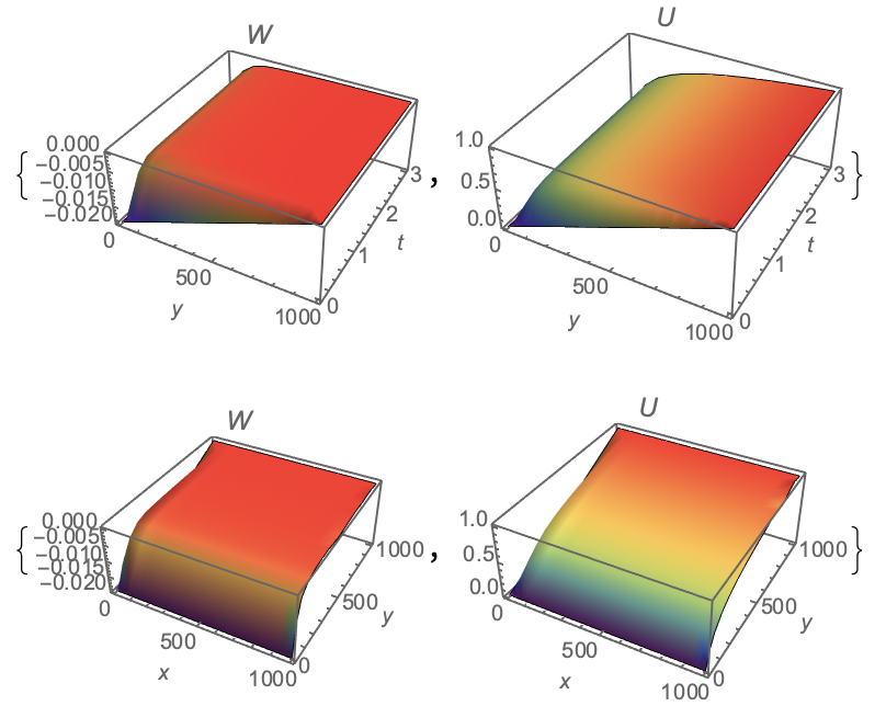
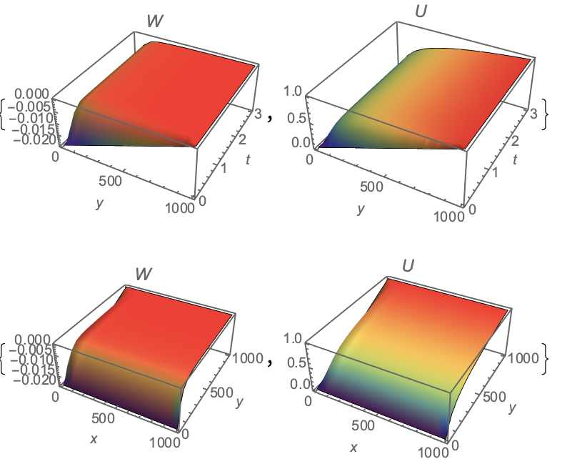
Visualisation
{Plot3D[W[L/2, y, t] /. First[sol], {y, 0, L}, {t, 0, T},
  PlotRange -> All, AxesLabel -> Automatic, PlotLabel -> W,
  Mesh -> None, ColorFunction -> "Rainbow"],
 Plot3D[u[L/2, y, t] /. First[sol], {y, 0, L}, {t, 0, T},
  PlotRange -> All, AxesLabel -> Automatic, PlotLabel -> U,
  Mesh -> None, ColorFunction -> "Rainbow"]}

{Plot3D[W[x, y, T] /. First[sol], {x, 0, L}, {y, 0, L},
  PlotRange -> All, AxesLabel -> {x, y, ""}, PlotLabel -> W,
  Mesh -> None, ColorFunction -> "Rainbow"],
 Plot3D[u[x, y, T] /. First[sol], {x, 0, L}, {y, 0, L},
  PlotRange -> All, AxesLabel -> {x, y, ""}, PlotLabel -> U,
  Mesh -> None, ColorFunction -> "Rainbow"]}
We see that both models describe the transition from a linear to a logarithmic profile in a finite time. We did not use bc1 in the last code, as this will increase the computing time several times with the same result. Why is time increasing?
#Update 1
I found a method to equalize computer time with bc1 and without bc1. It also allow us to answer the question. Code without bc1
 T = 3; L = 1000; W0 = .00002; U0 = 1;

 R = 13.22; px = 0.13; b = .0001; eq = \
{D[W[x, y, t], t] + u[x, y, t] D[W[x, y, t], x] +
    Integrate[W[x, y, t], {y, 0, y}]*D[W[x, y, t], y] -
    2*R*y*D[W[x, y, t], y] - R*(1 + y^2)*D[W[x, y, t], y, y] -
    D[W[x, y, t], x, x] == (y/(1 + y^2))*
     Integrate[W[x, y, t], {y, 0, y}] + b*y/(1 + y^2),
  D[u[x, y, t], t] + u[x, y, t] D[u[x, y, t], x] +
    Integrate[W[x, y, t], {y, 0, y}]*D[u[x, y, t], y] -
    R*y*D[u[x, y, t], y] - R*(1 + y^2)*D[u[x, y, t], y, y] -
    D[u[x, y, t], x, x] + px == 0};
ic = {W[x, y, 0] == W0*(y - L),
  u[x, y, 0] == U0*y/L}; bc = {W[x, L, t] == 0, W[x, 0, t] == -W0*L,
  W[0, y, t] == W0*(y - L), u[x, 0, t] == 0, u[x, L, t] == U0,
  u[0, y, t] == U0*y/L}; bc1 = {Derivative[1, 0, 0][u][L, y, t] == 0,
  Derivative[1, 0, 0][W][L, y, t] == 0};
 Dynamic["time: " <> ToString[CForm[currentTime]]]
AbsoluteTiming[
 sol = NDSolve[{eq, ic, bc}, {W, u}, {x, 0, L}, {y, 0, L}, {t, 0, T},
    Method -> {"MethodOfLines",
      "DifferentiateBoundaryConditions" -> False,
      "SpatialDiscretization" -> {"TensorProductGrid",
        "MinPoints" -> 150}},
    EvaluationMonitor :> (currentTime = t;)];]
Computational time {172.642, Null}, and we have a message
NDSolve::bcart: Warning: an insufficient number of boundary conditions have been specified for the direction of independent variable x. Artificial boundary effects may be present in the solution.
If we use homogeneous Neumann conditions at x=L= bc1, then the code is
Dynamic["time: " <> ToString[CForm[currentTime]]]
AbsoluteTiming[
 sol1 = NDSolve[{eq, ic, bc, bc1}, {W, u}, {x, 0, L}, {y, 0, L}, {t,
     0, T}, Method -> {"MethodOfLines",
      "DifferentiateBoundaryConditions" -> False,
      "SpatialDiscretization" -> {"TensorProductGrid",
        "MinPoints" -> 150}},
    EvaluationMonitor :> (currentTime = t;)];]
In this case we have computational time {167.784, Null}, and there are no messages. Now we must explain why, without option "DifferentiateBoundaryConditions" -> False, time increases several times. Here we solve a system of integro-differential equations. With option, the problem boils down to solving a system of algebraic equations. Without this option, the system is transformed into a system of differential equations that are solved together.
#Update 2
As suggested by @xzczd, we test code without integrals. Integrate[W[x, y, t], {y, 0, y}] is transformed into new function D[V[x,y,t],y]==W[x,y,t], and from it we derive an equation D[V[x, y, t], y, t] + D[V[x, y, t], y, x] == D[W[x, y, t], t] + D[W[x, y, t], x]. With this equation we solve a problem and compare with the code from Update 1 containing integrals. There is not much difference between the two solutions. New code:
T = 3; L = 1000; W0 = .00002; U0 = 1; R = 13.22; px = 0.13; b = \
.0001; eq = {D[W[x, y, t], t] + u[x, y, t] D[W[x, y, t], x] +
V[x, y, t]*D[W[x, y, t], y] - 2*R*y*D[W[x, y, t], y] -
    R*(1 + y^2)*D[W[x, y, t], y, y] -
    D[W[x, y, t], x, x] == (y/(1 + y^2))*V[x, y, t] + b*y/(1 + y^2),
  D[u[x, y, t], t] + u[x, y, t] D[u[x, y, t], x] +
    V[x, y, t]*D[u[x, y, t], y] - R*y*D[u[x, y, t], y] -
    R*(1 + y^2)*D[u[x, y, t], y, y] - D[u[x, y, t], x, x] + px == 0,
  D[V[x, y, t], y, t] + D[V[x, y, t], y, x] ==
   D[W[x, y, t], t] + D[W[x, y, t], x]};
ic = {W[x, y, 0] == W0*(y - L), u[x, y, 0] == U0*y/L,
  V[x, y, 0] == W0 (y^2/2 - L y)}; bc = {W[x, L, t] == 0,
  W[x, 0, t] == -W0*L, W[0, y, t] == W0*(y - L), u[x, 0, t] == 0,
  u[x, L, t] == U0, u[0, y, t] == U0*y/L};
bcV = {V[x, 0, t] == 0,
  V[0, y, t] ==
   W0 (y^2/2 - L y)}; bc1 = {Derivative[1, 0, 0][u][L, y, t] == 0,
  Derivative[1, 0, 0][W][L, y, t] == 0};
 Dynamic["time: " <> ToString[CForm[currentTime]]]
AbsoluteTiming[
 sol = NDSolve[{eq, ic, bc, bc1, bcV}, {W, V, u}, {x, 0, L}, {y, 0,
     L}, {t, 0, T},
    Method -> {"MethodOfLines",
      "DifferentiateBoundaryConditions" -> False,
      "SpatialDiscretization" -> {"TensorProductGrid",
        "MinPoints" -> 150}},
    EvaluationMonitor :> (currentTime = t;)];]
Update 3
Thanks to user21 remarks about SA model, I have modified bc for SA as
 bc = {nu[t, x, 0] == 0, u[t, x, 0] == 0, u[t, x, L] == 1,
   nu[t, x, L] == 0.1, nu[t, 0, y] == 0.1 y/L, u[t, 0, y] == y/L,
   Derivative[0, 1, 0][nu][t, L, y] == 0,
   Derivative[0, 1, 0][u][t, L, y] == 0};
With the Neumann boundary condition at x==L we have numerical solution without message from NDSolve. New solution for nu looks different from shown above




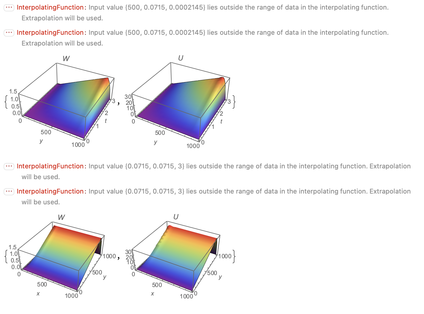
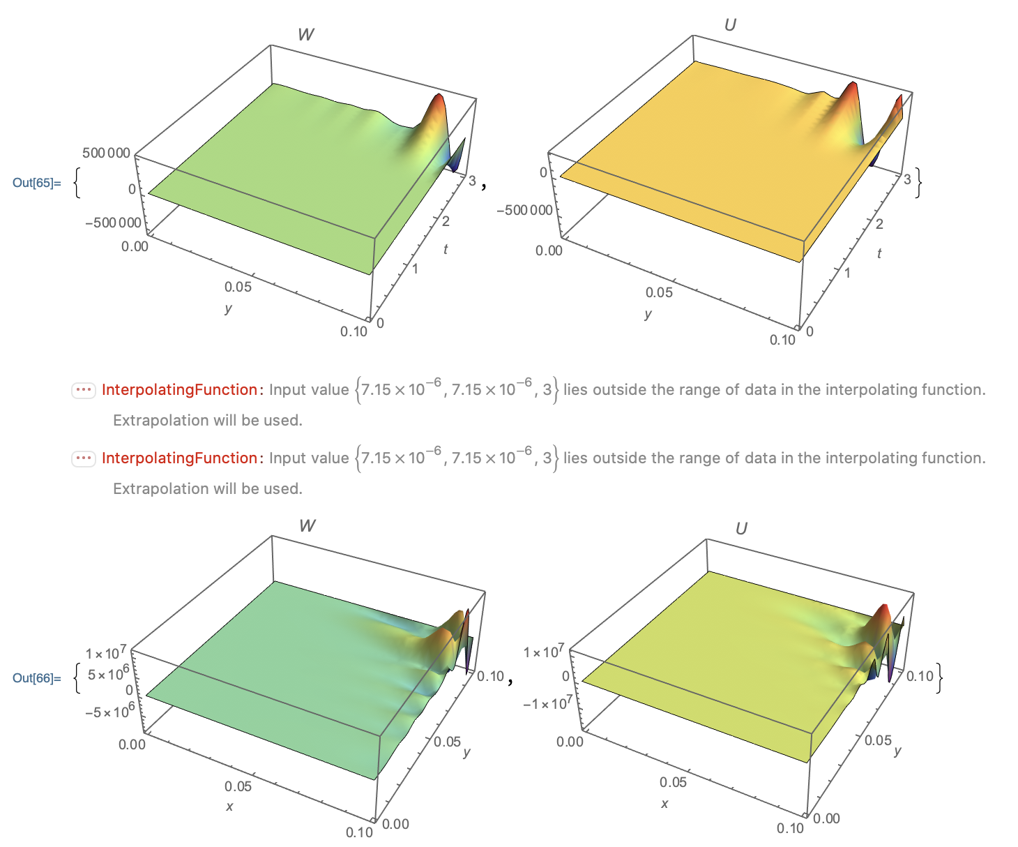
bc1works in v.12 with options, and in v.12.1 without options. Which version are you using? $\endgroup$MethodOfLinesaway. The third graphics looks rounded for small y. For larger t the values of W are lower. I tried Trace with NDSolve`MethodData reports Mathematica suggests, prefers LSODA for this problem if allow to select. The neat for the stepsize correction for the spatial error appears later. $\endgroup$bc1, although longer than withoutbc1. But in version 12.1, it only works without options on a coarse grid of 15 points. $\endgroup$TensorProductGrid, the zero Neumann value is automatically applied only forFiniteElementmethod. Please notice thebcartwarning is a serious problem. A detailed discussion can be found here: mathematica.stackexchange.com/q/73961/1871 $\endgroup$