Here is a variant of my chebInterpolation function for implementing piecewise Chebyshev interpolation.
ClearAll[chebInterpolation];
(* Constructs a piecewise InterpolatingFunction,
 * whose interpolating units are Chebyshev series *)
(* data0={{x0,x1},c1},..} *)
chebInterpolation[data0 : {{{_, _}, _List} ..}, {y0_, yp0_}] :=
  Module[{data = Sort@data0, domain1, coeffs1, domain, grid, ngrid,
    coeffs, order},
   domain1 = data[[1, 1]];
   coeffs1 = data[[1, 2]];
   domain = List @@ Interval @@ data[[All, 1]];
   grid = Union @@ data[[All, 1]];
   ngrid = Length@grid;
   coeffs = data[[All, 2]];
   order = Length[coeffs[[1]]] - 1;
   InterpolatingFunction[
     domain,
     {5, 1, order, {ngrid}, {order}, 0, 0, 0, 0, Automatic, {}, {},
      False},
     {grid},
     {{y0, yp0}}~Join~coeffs,
     {{{{1}}~Join~Partition[Range@ngrid, 2, 1]~
        Join~{{ngrid - 1, ngrid}}, {Automatic}~Join~
        ConstantArray[ChebyshevT, ngrid]}}
     ] /; Length[domain] == 1 && ArrayQ@coeffs];

Nx = 64; u0 = 0; uN = 5.0`100; du = (uN - u0)/Nx;
ugrid = Rescale[Sin[Pi/2 Range[-Nx, Nx, 2]/Nx], {-1, 1}, {u0, uN}];
C0 = Exp[-(# - uN/2)^2/2] &@ugrid;
dC0 = Evaluate@D[Exp[-(# - uN/2)^2/2], #] &@First@ugrid;
cc = Sqrt[2/Nx] FourierDCT[C0, 1];
cc[[{1, -1}]] /= 2;

C0Poly = chebInterpolation[N@{{{u0, uN}, cc}}, N@{First@C0, dC0}];
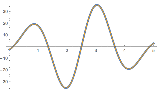
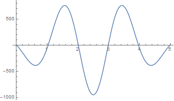
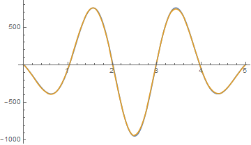
Plot of the 7th derivative:
Plot[{D[Exp[-(x - uN/2)^2/2], {x, 7}], D[C0Poly[x], {x, 7}]} //
  Evaluate, {x, u0, uN},
 PlotStyle -> {AbsoluteThickness[4], AbsoluteThickness[1.6]}]
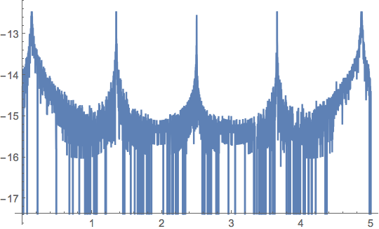
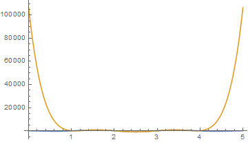
Log relative error of the 7th derivative:
Plot[{(D[C0Poly[x], {x, 7}] - D[Exp[-(x - uN/2)^2/2], {x, 7}])/
    Abs@D[Exp[-(x - uN/2)^2/2], {x, 7}]} // RealExponent //
  Evaluate, {x, u0, uN}]

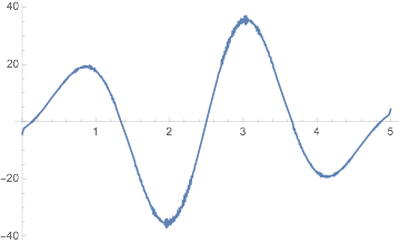
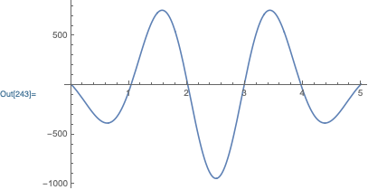


Lx? To plot derivative I would usePlot[D[C0Poly[\[FormalX]], {\[FormalX], 7}] /. \[FormalX] -> x, {x, 0, Lx}]. In help page onInterpolationOrder->Possibe issues it is written that "Very high-order interpolation can lead to large errors". $\endgroup$Method->"Spline". Sometimes the default"Hermite"has issues, esp. with derivatives. $\endgroup$