2
$\begingroup$

I've animated a dynamics as follows in Python. However, I'd like to have the same in Mathematica (whose graphics output, in my view, is fancier than Matplotlib).

#!/usr/bin/env python
# -*- coding: utf-8 -*- 

from scipy.integrate import odeint
import matplotlib.pyplot as plt
import numpy as np
import matplotlib as mpl
import mpl_toolkits.mplot3d.axes3d as p3
from matplotlib import animation
plt.style.use('seaborn-pastel')

def f(p, t): 
      x1 = p[0]
      y1 = p[1]
      x2 = p[2]
      y2 = p[3]
      dx1dt = x2 - x1
      dy1dt = y2 - y1
      dx2dt = x1 - x2
      dy2dt = y1 - y2
      return np.array ([dx1dt, dy1dt, dx2dt, dy2dt])

ts = np.arange (0 , 20 , 0.1)
x10 = -5
y10 = -7
x20 = -5
y20 = 7

p = np.array ([x10 , y10, x20 , y20])

s = odeint (f , p , ts)
x1s = s [: , 0]
y1s = s [: , 1]
x2s = s [: , 2]
y2s = s [: , 3] 

fig = plt.figure()
ax = p3.Axes3D(fig)

def update_lines(num, dataLines, lines):
    for line, data in zip(lines, dataLines):
        line.set_data(data[0:2, :num])
        line.set_3d_properties(data[2, :num])
        line.set_marker("o")
        #line.set_label("p1")
        #plt.legend()
    return lines

data = np.array([[x1s,y1s,ts],[x2s,y2s,ts]])

lines = [ax.plot(dat[0, 0:1], dat[1, 0:1], dat[2, 0:1])[0] for dat in data]

ax.set_xlim(-10.1,10.1)
ax.set_ylim(-10.1,10.1)
ax.set_zlim(0,20)
ax.set_xlabel("x")
ax.set_ylabel("y")
ax.set_zlabel("t")
ax.legend()

anim = animation.FuncAnimation(fig, update_lines, 50, fargs=(data, lines),
                                   interval=200, blit=True, repeat=True)

plt.rcParams['animation.ffmpeg_path'] ='C:\\...\\FFmpeg\\bin\\ffmpeg.exe'
FFwriter = animation.FFMpegWriter(fps = 100)
anim.save('test.mp4', writer = FFwriter)
                                                   
plt.show()

As a newbie in using Mathematica, here is what I have planned to recreate the animation above.

1- Numerically integrating the system using DSolve[]

DSolve[{x1'[t] == -x1[t] + x2[t], 
  y1'[t] == -y1[t] + y2[t], 
  x2'[t] == x1[t] - x2[t], 
  y2'[t] == y1[t] - y2[t], -5, -7, -5, 7}, x1[t], y1[t],
  x2[t], y2[t], t]

2- Animating the integration result using Animate[Plot3D[...]]

But, I don't know how to set variation ranges corresponding to my variables. Can you please give a clue?


Edit:

The desired script does numerically integrate the following system of equations

dx1dt = x2 - x1
dy1dt = y2 - y1
dx2dt = x1 - x2
dy2dt = y1 - y2

According to the initial conditions below

x10 = -5
y10 = -7
x20 = -5
y20 = 7

Then the overall dynamics of the system is animated by varying the time t between $0$ to $20$ units.

$\endgroup$
4
  • 2
    $\begingroup$ Can you please explain what your script is doing and what is the desired result for all those who do not speak python. $\endgroup$
    – yarchik
    Commented Jul 21, 2019 at 12:42
  • $\begingroup$ @yarchik: Please check the edit $\endgroup$
    – user66658
    Commented Jul 21, 2019 at 12:46
  • $\begingroup$ I still do not understand. You solve ODE for 4 functions. They all depend on t. How do you make a 3D plot out of them? 3D plot needs one 1 function that depends on 2 parameters. $\endgroup$
    – yarchik
    Commented Jul 21, 2019 at 12:59
  • $\begingroup$ @yarchik: The result is actually the trajectories of the simulated agents. What is actually drawn is a set of tuples (x,y,t) in a 3D space. $\endgroup$
    – user66658
    Commented Jul 21, 2019 at 13:02

2 Answers 2

4
$\begingroup$

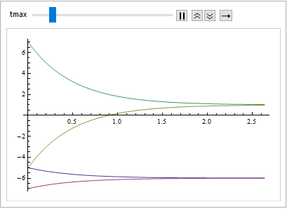
You can use NDSolveValue and Animate:

ClearAll[x1, x2, y1, y2]
ndsv = NDSolveValue[{x1'[t] == -x1[t] + x2[t], 
    y1'[t] == -y1[t] + y2[t], 
    x2'[t] == x1[t] - x2[t], 
    y2'[t] == y1[t] - y2[t], 
    x1[0] == -5, x2[0] == -7, y1[0] == -5,  y2[0] == 7}, 
   {x1, x2, y1, y2}, 
   {t, 0, 20}, 
   "ExtrapolationHandler" -> {Undefined &, "WarningMessage" -> False}];


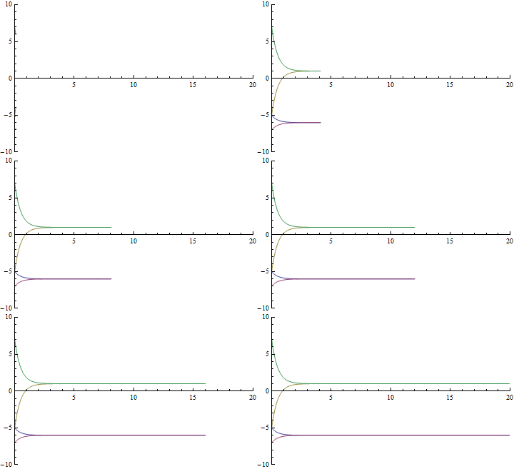
Animate[Plot[Evaluate@Through@ndsv[t], {t, 0, tmax}], {tmax, .1, 20}]

enter image description here

frames = Table[Plot[Evaluate@Through@ndsv[t], {t, 0, tmax}], {tmax, .1, 20, .1}];

Export["frms.gif", frames]

enter image description here

frames2 = Table[Plot[Evaluate@Through@ndsv[t], {t, 0, tmax}, 
    PlotRange -> {{0, 20}, {-10, 10}}], {tmax, .1, 20, .1}];

Export["frms2.gif", frames2]

enter image description here

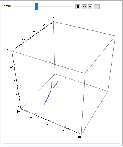
Update: For 3D visualization, you can use ParametricPlot3D with {{x1[t], y1[t], t}, {x2[2], y2[t], t}} as the first argument:

Animate[ParametricPlot3D[{{ndsv[[1]]@t, ndsv[[3]]@t, t}, 
    {ndsv[[2]]@t, ndsv[[4]]@t, t}}, {t, 0, tmax}, 
  BoxRatios -> 1,  BaseStyle -> Thick, PlotRange -> {{-10, 10}, {-10, 10}, {0, 20}}], 
 {tmax, .1, 20}]

enter image description here

$\endgroup$
5
  • $\begingroup$ Thanks, but the result needs to be 3D, say, $(x,y,t)$ points. $\endgroup$
    – user66658
    Commented Jul 21, 2019 at 13:06
  • $\begingroup$ @Roboticist, for the error message add ClearAll[x1,x2, y1,y2] before the code. $\endgroup$
    – kglr
    Commented Jul 21, 2019 at 13:09
  • 1
    $\begingroup$ @Roboticist, for 3D visualization please see the update. $\endgroup$
    – kglr
    Commented Jul 21, 2019 at 13:19
  • $\begingroup$ I do appreciate your help! $\endgroup$
    – user66658
    Commented Jul 21, 2019 at 13:19
  • 1
    $\begingroup$ @Roboticist, my pleasure. Welcome to mma.se. $\endgroup$
    – kglr
    Commented Jul 21, 2019 at 13:20
1
$\begingroup$

The OP mentions "numerically integrating...using DSolve[]." DSolve[] does a symbolic integration, which I will show, and I will also show numerical integration using NDSolve[], which can used to construct a faster (more responsive) Animate[]/Manipulate[] visualization (because all of the points are pre-calculuated and stored).

Symbolic solution:

ClearAll[x1, x2, y1, y2, t]
dsol = DSolveValue[  (* integrate *)
  {x1'[t] == -x1[t] + x2[t], y1'[t] == -y1[t] + y2[t], 
   x2'[t] == x1[t] - x2[t], y2'[t] == y1[t] - y2[t], x1[0] == -5, 
   x2[0] == -7, y1[0] == -5, y2[0] == 7},
  {x1, y1, x2, y2}, {t, 0, 20}]
(*
  {Function[{t}, -6 + E^(-2 t)], Function[{t}, 1 - 6 E^(-2 t)], 
   Function[{t}, -6 - E^(-2 t)], Function[{t}, 1 + 6 E^(-2 t)]}
*)

P1 = Function[t, Evaluate[Flatten@{t, Through[dsol[[{1, 2}]][t]]}]]
P2 = Function[t, Evaluate[Flatten@{t, Through[dsol[[{3, 4}]][t]]}]]
(* 
  Function[t, {t, -6 + E^(-2 t), 1 - 6 E^(-2 t)}]
  Function[t, {t, -6 - E^(-2 t), 1 + 6 E^(-2 t)}]
*)

Animate[
 ParametricPlot3D[{P1[tt], P2[tt]}, {tt, 0, t + $MachineEpsilon}, 
  PlotRange -> {{0, 20}, {-11, -1}, {-5, 7}}, 
  PlotRangePadding -> Scaled[0.05],
  (* Manipulate/Animate localize t which gives it a ugly symbol name *)
  (* The string processed by ToExpression won't be mapped to the local var. *)
  (* One could simply use strings, but 
  (*   this way, you get the nice italic look of TraditionalForm *)
  AxesLabel -> (ToExpression[#, StandardForm, HoldForm] & /@ {"t", "x", "y"})],
 {t, 0, 20}
 ]

Numerical solution:

The trick here is to construct the integral curves from the values computed by NDSolve[] (NDSolveValue[] is just syntactic sugar for NDSolve[]). The evolution of the integral curve can be done by selecting an initial segment of each curve up to the current animation time.

ndsol = NDSolveValue[{
    x1'[t] == -x1[t] + x2[t], y1'[t] == -y1[t] + y2[t], 
    x2'[t] == x1[t] - x2[t], y2'[t] == y1[t] - y2[t], x1[0] == -5, 
    x2[0] == -7, y1[0] == -5, y2[0] == 7,
    tt'[t] == 1, tt[0] == 0},  (* dummy int. to get time steps more easily *)
   {x1, y1, x2, y2, tt}, {t, 0, 20}];

(* get points from values computed by NDSolve[] *)
(* xy coords. of pt. 1 are parts {1, 2}, of pt. 2 are parts {3, 4}; time is part 5 *)
values = Through[ndsol["ValuesOnGrid"]];
points = {Transpose@values[[{5, 1, 2}]], Transpose@values[[{5, 3, 4}]]};

(* make a nicely scaled PlotRange - I cheated and also used this above *)
plotrng = Apply[{#5, MinMax[{#1, #3}], MinMax[{#2, #4}]} &, MinMax /@ values];
With[{m = Max[-Subtract @@@ plotrng]},
 plotrng =    (* expand zero-length ranges -- not needed in this specific case *)
  plotrng /. {a1_Real, a2_Real} /; a2 == a1 :> {a1 - 0.5 m, a2 + 0.5 m};
 plotrng = Rescale[#, Mean[#] - Subtract @@ # {-1, 1}, 
     Mean[#] + Max[0.5 m, -Subtract @@ #] {-1, 1}] & /@ plotrng
 ]
(*  {{0., 20.}, {-11., -1.}, {-5., 7.}}  *)

Animate[
 Graphics3D[
  {Thick, Riffle[
    ColorData[97] /@ Range@2,
    Line /@ points[[All, ;; LengthWhile[values[[5]], # <= t &]]] (* segments of curves *)
    ]},
  PlotRange -> plotrng, PlotRangePadding -> Scaled[0.05],
  Boxed -> True, Axes -> True,
  AxesLabel -> (ToExpression[#, StandardForm, HoldForm] & /@ {"t", "x", "y"})
  ],
 {t, Sequence @@ plotrng[[1]]}
 ]

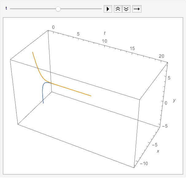
Both animations produce an output like the one below. The second is more responsive because there is very little computation compared to ParametricPlot3D.

enter image description here

$\endgroup$

Your Answer

By clicking “Post Your Answer”, you agree to our terms of service and acknowledge you have read our privacy policy.