3
$\begingroup$

What I want to get is a density plot where the color function is thresholded: if the value of a function is larger a threshold, the color function returns white; otherwise, black.

I found some tutorials about how to create gradient color functions, but didn't find one for any thresholded color function.

If any of you teach this, it would be greatly appreciated.

$\endgroup$

3 Answers 3

7
$\begingroup$

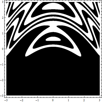
Update: An alternative way to use ContourPlot using threshold as the single Contour with the option ContourShading:

threshold = .5;    
ContourPlot[FractionalPart[y + Sin[x^2 + 3 y]], {x, -3, 3}, {y, -3, 3}, 
  Contours -> {threshold}, ContourShading -> {Black, White}, 
  Exclusions -> None, PlotPoints -> 90] 

enter image description here

Similarly, DensityPlot with MeshFunctions, Mesh and MeshShading options:

DensityPlot[FractionalPart[y + Sin[x^2 + 3 y]], {x, -3, 3}, {y, -3, 3}, 
 MeshFunctions -> {#3 &}, Mesh -> {{threshold}}, 
 MeshShading -> {Black, White}, PlotPoints -> 90, 
 Exclusions -> None, WorkingPrecision -> 10] 

enter image description here

And, a combination of Raster and Image:

Image @ Raster[Table[UnitStep[FractionalPart[y + Sin[x^2 + 3 y]] - threshold], 
 {y, -3, 3,  1/100}, {x, -3, 3, 1/100}]]

enter image description here

We get the same picture using Boole[FractionalPart[y + Sin[x^2 + 3 y]] >= threshold] instead of UnitStep[FractionalPart[y + Sin[x^2 + 3 y]] - threshold].

Original answer:

You can use ContourPlot with options Contours and ContourShading:

threshold = .5;
ContourPlot[y + Sin[x^2 + 3 y], {x, -3, 3}, {y, -3, 3}, 
  Contours -> {threshold}, ContourShading -> {Black, White}]
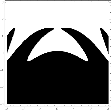
enter image description here

Another alternative is to use RegionPlot:

RegionPlot[y + Sin[x^2 + 3 y] <= threshold, {x, -3, 3}, {y, -3, 3} , 
 BoundaryStyle -> Black, PlotStyle -> Black, PlotPoints -> 100]

enter image description here

With DensityPlot you can do

DensityPlot[y + Sin[x^2 + 3 y] , {x, -3, 3}, {y, -3, 3}, 
  ColorFunction -> (Black &), RegionFunction -> (#3 <= threshold &)] 
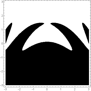
enter image description here

You can also use DensityPlot with the option ColorFunction with large enough value for PlotPoints to get a similar picture the one above:

cf1 = If[# <= threshold, Black, White] &;
DensityPlot[y + Sin[x^2 + 3 y], {x, -3, 3}, {y, -3, 3}, 
  ColorFunction -> cf1, PlotPoints -> 250]

enter image description here

Using cf2 = Blend[{Black, White}, UnitStep[# - threshold]] &; in place of cf1 gives the same result.

$\endgroup$
7
  • $\begingroup$ As a curiosity, why Density plot is less clear than ContourPlot in general? $\endgroup$ Commented Sep 22, 2018 at 23:13
  • 1
    $\begingroup$ @TaikiBessho, I meant the blending of colors, for example, DensityPlot[y + Sin[x^2 + 3 y], {x, -3, 3}, {y, -3, 3}, ColorFunction -> (If[# <= threshold, Black, White] &)] unless you use some additional trick. $\endgroup$
    – kglr
    Commented Sep 22, 2018 at 23:22
  • 1
    $\begingroup$ @TaikiBessho, you might want to add the option MaxRecursion with a high enough value (say 7) to DensityPlot and RegionPlot. I don't know the internal workings of ContourPlot`. $\endgroup$
    – kglr
    Commented Sep 23, 2018 at 19:37
  • 1
    $\begingroup$ Wait, the results given by the first 2 samples are wrong, aren't they?: Plot[FractionalPart[y + Sin[x^2 + 3 y]] /. x -> 0 // Evaluate, {y, -3, 3}] $\endgroup$
    – xzczd
    Commented Oct 1, 2018 at 8:01
  • 1
    $\begingroup$ Thank you @xzczd; adding Exclusions->None fixed the issue. $\endgroup$
    – kglr
    Commented Oct 1, 2018 at 8:22
3
$\begingroup$

You may consider Image and Binarize:

expr = FractionalPart[y + Sin[x^2 + 3 y]];

Binarize[Image@Reverse@Transpose@Table[expr, {x, -3, 3, 0.01}, {y, -3, 3, 0.01}], 0.5]

If you need the frame, ArrayPlot and UnitStep may be a better choice:

frame = DensityPlot[, {x, -3, 3}, {y, -3, 3}];

binarize = {x, threshold} \[Function] 
           Evaluate@Simplify`PWToUnitStep@Piecewise[{{1, x < threshold}}]

frame~Show~ArrayPlot[
  binarize[Table[expr, {x, -3, 3, 0.01}, {y, -3, 3, 0.01}]\[Transpose], 0.5], 
  DataReversed -> True, DataRange -> {{-3, 3}, {-3, 3}}]

Mathematica graphics

$\endgroup$
3
$\begingroup$

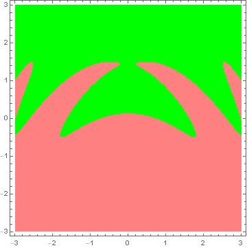
If one really wishes to use DensityPlot[] (even tho the other answers have already shown better approaches), you need to remember to set ColorFunctionScaling -> False before using a thresholded color function. In the following example, I combine GrayLevel[] and UnitStep[]:

With[{h = 1/2},
     DensityPlot[y + Sin[x^2 + 3 y], {x, -3, 3}, {y, -3, 3}, 
                 ColorFunction -> Function[z, GrayLevel[UnitStep[z - h]]], 
                 ColorFunctionScaling -> False, PlotPoints -> 205]]

monochrome thresholded plot

More generally, one can use Blend[] and Boole[] for such plots:

With[{h = 1/2},
     DensityPlot[y + Sin[x^2 + 3 y], {x, -3, 3}, {y, -3, 3}, 
                 ColorFunction -> Function[z, Blend[{Pink, Green}, Boole[z > h]]], 
                 ColorFunctionScaling -> False, PlotPoints -> 205]]

colored version

$\endgroup$

Your Answer

By clicking “Post Your Answer”, you agree to our terms of service and acknowledge you have read our privacy policy.

Not the answer you're looking for? Browse other questions tagged or ask your own question.