Solving a system of ODEs with the Runge-Kutta method

Question

I'm trying to solve a system of ODEs using a fourth-order Runge-Kutta method. I have to recreate certain results to obtain my degree. But I'm a beginner at Mathematica programming and with the Runge-Kutta method as well.

{A = 0.30, B = 1, C = 40, D = 1, E = 0.75, F = 0.11,
 r = 2.5, a = 2, e = 0.475, g = 2, d = 0.03, n = 0.01, p = -0.00005}

x'[t]/x[t] = (A + B x[t] - C x[t]^2 - F)/(D + E^(r y[t]));   
y'[t]/y[t] = g (((a s[t] x[t] k[t])/m[t]) - e) (1 - y[t]); 
m'[t]/m[t] = n;
k'[t]/k[t] = x[t] - d;
s'[t]/s[t] = -p;

I'd appreciate any kind of help. For over a month now, I've tried to solve this system myself but have only gotten bad results. This model is supposed to fluctuate around the equilibrium point, but in the code I have so far, this doesn't happen.

Answer 1

Here is a functional approach. The following will give you one step of the Runge-Kutta formula:

RungeKutta[func_List, yinit_List, y_List, step_] := 
 Module[{k1, k2, k3, k4},
  k1 = step N[func /. MapThread[Rule, {y, yinit}]];
  k2 = step N[func /. MapThread[Rule, {y, k1/2 + yinit}]];
  k3 = step N[func /. MapThread[Rule, {y, k2/2 + yinit}]];
  k4 = step N[func /. MapThread[Rule, {y, k3 + yinit}]];
  yinit + Total[{k1, 2 k2, 2 k3, k4}]/6]

Here, func is a list of functions, yinit a list of initial values, y a list of function variables (in your case that will be {x, y, m, k, s}, and step is the step size of the numerical simulation. You can then use something like NestList to iterate it many times like this:

NestList[RungeKutta[func, #, y, step] &, N[yinit], Round[t/step]]

Here, t is the maximum value of your independent variable. You can also include conditionals to check that the lists are of equal length.

Answer 2

andre has linked you to the method plug-in framework in the comments, but there is a more direct way to implement classical Runge-Kutta, just by supplying its Butcher tableau to "ExplicitRungeKutta". Here's an adaptation from the docs:

ClassicalRungeKuttaCoefficients[4, prec_] := With[{amat = {{1/2}, {0, 1/2}, {0, 0, 1}},
           bvec = {1/6, 1/3, 1/3, 1/6}, cvec = {1/2, 1/2, 1}}, N[{amat, bvec, cvec}, prec]]

{xf, yf} = {x, y} /. First @ 
           NDSolve[{x'[t] == -y[t], y'[t] == x[t], x[0] == 1, y[0] == 0},
                   {x, y}, {t, 0, 6}, 
                   Method -> {"ExplicitRungeKutta", "DifferenceOrder" -> 4,
                              "Coefficients" -> ClassicalRungeKuttaCoefficients},
                   StartingStepSize -> 1/2];

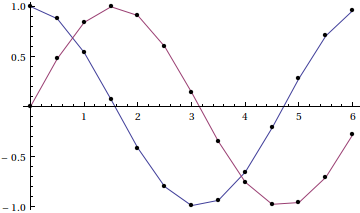
To obtain the values computed by RK, you can then do this:

xl = MapThread[Append, {xf["Grid"], xf["ValuesOnGrid"]}]
   {{0., 1.}, {0.5, 0.877604}, {1., 0.540588}, {1.5, 0.0714256}, {2., -0.415108},
    {2.5, -0.800012}, {3., -0.989166}, {3.5, -0.936349}, {4., -0.65453}, {4.5, -0.212684},
    {5., 0.281088}, {5.5, 0.706007}, {6., 0.95816}}

yl = MapThread[Append, {yf["Grid"], yf["ValuesOnGrid"]}]
   {{0., 0.}, {0.5, 0.479167}, {1., 0.841037}, {1.5, 0.99713}, {2., 0.90931},
    {2.5, 0.599108}, {3., 0.142441}, {3.5, -0.348969}, {4., -0.754924}, {4.5, -0.976153},
    {5., -0.958587}, {5.5, -0.706572}, {6., -0.281796}}

Plot them:

ListLinePlot[{xl, yl}, Mesh -> All, MeshStyle -> PointSize[Medium]]

Answer 3

First of all, I'd like to emphasize that, if you just want to solve an initial value problem (IVP) of ordinary differential equation (ODE) or ODE system, please use NDSolve. Forget about the classical Runge-Kutta (classical RK, RK4), it's mainly for pedagogical purposes nowadays, and not comparable to the default method of NDSolve at all. If default method of NDSolve fails to solve your IVP, RK4 won't save your day, either. Actually I've never seen a knotty problem solved by switching from default NDSolve method to RK4 since I began using Mathematica 10 years ago.

If you need RK4 for certain special reason (e.g. to exactly reproduce numeric result obtained with RK4 in literature, to ensure the result can be easily reproduced by others, etc.), setting proper options for NDSolve is the way to go. Please refer to J.M.'s answer for more info. Here I'll provide a general-purposed package for setting up explicit Runge-Kutta method with no adaptive step control, which is implemented without the help of NDSolve, just for fun:

BeginPackage["primaryRK`"];
rkstepgenerator; rhsfuncgenerator; rk4stepfunc;
Begin["`private`"];

rule = {semi -> CompoundExpression, set -> Set, 
        module -> Module, compile -> Compile};
SetAttributes[semi, Flat];
f[{}, _] := {};

rkstepgenerator[a_, b_, c_] := (s = Length@b;
  k = ToExpression["k" <> ToString@#] & /@ Range@s;
  Function @@ {f, 
     compile[{t, {y, _Real, 1}, dt}, 
      module[k, semi[
        semi @@ Thread@
          set[k, Prepend[Thread@f[t + c dt, y + dt k . PadRight[#, s] & /@ a], 
            f[t, y]]],
        y + dt b . k]]]} /. rule)

a = {{1/2}, {0, 1/2}, {0, 0, 1}};
b = {1/6, 1/3, 1/3, 1/6};
c = {1/2, 1/2, 1};

rk4stepfunc = rkstepgenerator[a, b, c];

rhsfuncgenerator[t_, ylst_][expr_] := 
 Function @@ {{t, yvec}, module[ylst, semi[ylst~set~yvec, expr]]} /. rule

End[];
EndPackage[]

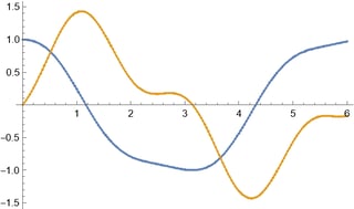
Since RK4 is so frequently requested, a function rk4stepfunc is included in the package. Let me use the IVP

\begin{aligned}x'(t)&=-y(t)\\ y'(t)&=x(t)+\sin(3t)\\ x(0)&=1\\ y(0)&=0\end{aligned}

to illustrate its possible usage:

heads = {x, y}; 
vars = heads[t] // Through;
eqs = {x'[t] == -y[t], y'[t] == x[t] + Sin[3 t]};
iclst = {1, 0};
domain = {t0, tend} = {0, 6};

(* Analytic solution for comparison: *)
ref = Plot[
        vars /. DSolve[{eqs, vars == iclst /. t -> t0}, vars, t] // 
        Evaluate, {t, t0, tend}];

expr = 
  Solve[eqs, D[vars, t]][[1, All, -1]] /. 
    (h : Alternatives @@ heads)[t] :> h
(* {-y, x + Sin[3 t]} *)

Internal`$ContextMarks = False; (* Default value is Automatic *)

rhsfunc = rhsfuncgenerator[t, heads]@expr
(* Function[{t, yvec}, Module[{x, y}, {x, y} = yvec; {-y, x + Sin[3 t]}]] *)

step = rk4stepfunc@rhsfunc;

dt = 1/30;
tlst = Range[t0, tend, dt];

sollst = 
   FoldList[step[#2[[1]], #, #2[[2]]] &, iclst, 
    Transpose@{Most@tlst, Differences@tlst}]; // AbsoluteTiming
(* {0.0013601, Null} *)

ListPlot[Thread /@ Thread@{tlst, sollst} // Transpose]~Show~ref

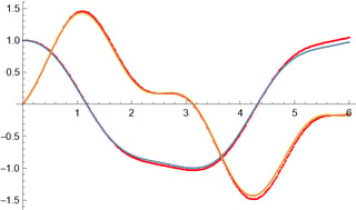
You can of course use the package to set up other explicit Runge-Kutta method with no error estimation e.g. explicit Euler. Just for fun, let me show another possible usage of the package:

eulerstepfunc = rkstepgenerator[{{}}, {1}, {}]
(* Function[f, 
            Compile[{t, {y, _Real, 1}, dt}, 
                    Module[{k1}, k1 = f[t, y]; dt k1 + y]]] *)

step = eulerstepfunc@rhsfunc;
dt = 1/50;
ti = t0 - dt;
sollst = NestList[
        step[ti = ti + dt, #, dt] &, iclst, #2 - # & @@ domain/dt // 
     Round]; // AbsoluteTiming
(* {0.0007594, Null} *)
ListPlot[sollst\[Transpose], DataRange -> domain, PlotStyle -> Red]~Show~ref

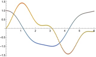
Heun's method (Once again, I'll show a different usage of the package for fun):

heunstepfunc = 
 With[{α = 1}, 
  rkstepgenerator[{{α}}, {1 - 1/(2 α), 1/(2 α)}, {α}]]
(* Function[f, 
 Compile[{t, {y, _Real, 1}, dt}, 
         Module[{k1, k2}, k1 = f[t, y]; 
                          k2 = f[dt + t, dt k1 + y]; 
                          dt (k1/2 + k2/2) + y]]] *)

step = heunstepfunc@rhsfunc;
sollst = With[{dt = 1/20, t0 = N@t0, step = step, iclst = N@iclst}, 
           With[{n = 1 - Subtract @@ domain/dt},
            Compile[{}, Module[{lst = Table[iclst, {n}], ti = t0},
                Do[lst[[i]] = step[ti, lst[[i - 1]], dt];
                   ti = ti + dt, {i, 2, n}];
                lst]]]][]; // AbsoluteTiming

Show[sollst\[Transpose] // 
  ListPlot[#, DataRange -> domain, ColorFunction -> "Rainbow"] &, ref]