Problems encoding a Bayesian Network when using MultinomialDistribution

Question

Short description of the encountered problem

I am getting an error when using a MultinomialDistribution to encode a conditional probability distribution (CPD) within the joint probability distribution of a Bayesian Network while it works completely fine as a standalone distribution. A bug?

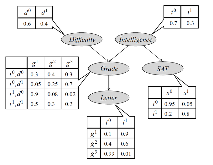
A simple Bayesian Network taken from Daphne Koller's book on PGM

As a minimal example, I am trying to encode the first three nodes of the Bayesian Network that is given on page 53 in Probabilistic Graphical Models (2009), by Daphne Koller and Nir Friedman:

Encoding the joint Probability Distribution P(I,D,G)

I am encoding the Bayesian Network given by the nodes Difficulty (easy,hard) of the class taken by a student, Intelligence (low,high) of the student and Grade (g1=A, g2=B, g3=C) achieved in the class as follows:

distI = BernoulliDistribution[ 0.3 ]; (* probability of high intelligence *)
distD = BernoulliDistribution[ 0.4 ]; (* probability of hard class *)

grade = Function[ { g1, g2, g3 },
    { g1, g2, g3 }.Range[3]
]; (* map the vector of grades onto the set {1,2,3} *)

(* conditional distribution of the grade *)
cpdG = Function[ { i, d },
    With[
      {
        n = 1,
        p = Piecewise[
                {
                  { {  0.3,  0.4, 0.3  }, i == 0 && d == 0 },
                  { { 0.05, 0.25, 0.7  }, i == 0 && d == 1 },
                  { {  0.9, 0.08, 0.02 }, i == 1 && d == 0 },
                  { {  0.5,  0.3, 0.2  }, i == 1 && d == 1 }
                }
            ]
      },
      TransformedDistribution[ 
          grade @@ {g1,g2,g3}, 
          {g1,g2,g3} \[Distributed] MultinomialDistribution[ n, p ]
      ]
    ]
];

(* the joint distribution P(I,D,G) as given by the chain rule *)
distB = ProbabilityDistribution[
    PDF[ distI, i] PDF[ distD, d] PDF[ cpdG[ i, d ], g ],
    {i, 0, 1, 1},
    {d, 0, 1, 1},
    {g, 1, 3, 1}
]

But this will give the follwing error message (repeatedly):

Note, that the conditional distribution nicely works on its own:

PDF[ cpdG[1, 1], 2 ]

0.3

What is the problem here?

Update

The MultinomialDistribution can be replaced with the EmpiricalDistribution, which avoids some problems:

(* conditional distribution of the grade *)
cpdG = Function[ { i, d },
    With[
      {
        p = Piecewise[
                {
                  { {  0.3,  0.4, 0.3  }, i == 0 && d == 0 },
                  { { 0.05, 0.25, 0.7  }, i == 0 && d == 1 },
                  { {  0.9, 0.08, 0.02 }, i == 1 && d == 0 },
                  { {  0.5,  0.3, 0.2  }, i == 1 && d == 1 }
                }
            ]
      },
      EmpiricalDistribution[ p -> Range[3] ]
    ]
];

Then we do probabilistic inference using Probability:

Probability[ g == 1 \[Conditioned] i == 1, {i,d,g} \[Distributed] distB ]

0.74

But to my disappointment this will fail for the full Bayesian Network -- but that should probably go into a separate question...

Answer 1

Explanation and Solution given by WRI support

I just received an answer from support:

What seems to be the issue is the Piecewise definition in cpdG. When evaluating ProbabilityDistribution[...], the values for i,d, and g are substituted after the definition is made, so the Piecewise definition remains general, which conflicts with the MultinomialDistribution. This also explains why the conditional distribution ( such as PDF[cpdG[1,1],2] ) works. Since the values for the variables are known, the piecewise definition within cpdG does not conflict with the MultinomialDistribution.

The solution proposed is the following:

We can get around this by defining a function that takes i,d, and g as arguments, and returns the value of cpdG for the desired input variables.

cpdGtable[ i_, d_, g_ ] := Table[
    PDF[ cpdG[i, d], g ], 
    {i, 0, 1, 1}, {d, 0, 1, 1}, {g, 1, 3, 1}
]

distB = ProbabilityDistribution[
    PDF[distI, i] PDF[distD, d] cpdGtable[i,d,g],
    {i,0,1,1},{d,0,1,1},{g,1,3,1}
];

Unfortunately this approach does not seem to work out as intended:

Probability[ g == 1, {i,d,g} \[Distributed] distB ]

{{{0.3, 0.4, 0.3}, {0.05, 0.25, 0.7}}, {{0.9, 0.08, 0.02}, {0.5, 0.3, 0.2}}}

Alternate Solution using Indicator Functions

As the use of Piecewise seems to be an issue when using MultinomialDistribution using Boole instead will work:

(* code up to this point as in the OP *)
cpdG = Function[ {i, d},
    With[
      {
        n = 1,
        p = Plus[
              {0.3 , 0.4 , 0.3}  Boole[i==0 && d==0],
              {0.05, 0.25, 0.7}  Boole[i==0 && d==1],
              {0.9 , 0.08, 0.02} Boole[i==1 && d==0],
              {0.5 , 0.3 , 0.2}  Boole[i==1 && d==1]
            ]
      },
      TransformedDistribution[ 
        grade@@{g1,g2,g3},
        {g1,g2,g3} \[Distributed] MultinomialDistribution[n,p]
      ]
    ]
];

distB = ProbabilityDistribution[
   PDF[distI, i] PDF[distD, d] PDF[cpdG[i, d], g], 
   {i, 0, 1, 1}, {d, 0, 1, 1}, {g, 1, 3, 1}
];

Now everything works out fine, and the probability for getting an A given a high IQ turns out to be 74%:

Probability[ g==1 \[Conditioned] i==1, {i,d,g} \[Distributed] distB ]

0.74

UPDATE

We can get around this by defining a function that takes i,d, and g as arguments, and returns the value of cpdG for the desired input variables.

While it has been awhile, I lately came back to this question and we can indeed make the original approach work out by making sure, that the PDF within ProbabilityDistribution is defined with concise values, i.e., we have to make sure it is not evaluate too soon.

A very simple and straightforward apporach is to define a function cpdfG which will provide the correct PDF for node G when it is given numerical values:

cpdfG[ i_?NumericQ, d_?NumericQ, g_?NumericQ ] := With[
    { dist = cpdG[ i, d ] }
    ,
    PDF[ dist, g ]
]

Leaving everything as given in the original post, we define the joint probability distribution as follows:

distB = ProbabilityDistribution[
    PDF[ distI, i] PDF[ distD, d] cpdfG[ i, d, g ],
    {i, 0, 1, 1},
    {d, 0, 1, 1},
    {g, 1, 3, 1}
]

Probability[ g == 1, {i, d, g} \[Distributed] distB ]

(* 0.362 *)