Need help with making an interactive 3D plot

Question

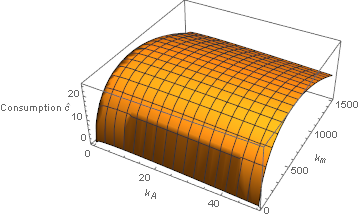
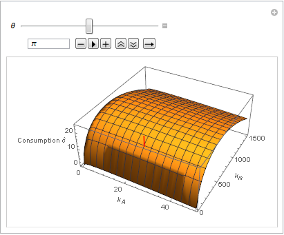
My main problem is to generate a manipulatable 3D plot, combining three functions and two of those functions depend on another variable Theta (which shall be the manipulateable variable). To explain it in detail:

I have two functions, which depend on the variable Theta. The variable Theta shall later be the factor which can be manipulated. So at first I defined two functions (kbA and kbM), which depend on this variable:

No. 1)

CPA[ϕ_, α_, β_, δ_, x_, ρ_, θ_, kM_] := 
  cA[t]*ϕ*(α kA^(α - 1) + β kM^(β - 1) - δ - ρ - x θ)/θ

kbA = kA /.  Flatten@Solve[
CPA[0.5, 1/3, 2/3, 0.05, 0.02, 0.01, θ, 500] == 0.0, kA]

No. 2)

CPM[ϕ_, α_, β_, δ_, x_, ρ_, θ_, kA_] := 
  cM[t]*(1 - ϕ )*(α kA^(α - 1) + β kM^(β - 1) - δ - ρ - x θ)/θ

kbM = kM /. Flatten@Solve[CPM[0.5, 1/3, 2/3, 0.05, 0.02, 0.01, θ, 500] == 0.0, kM]

Those two functions (kbA and kbM) depend on Theta. (The results, kA* and kM*, of these functions theoretically define two coordinate values for a line plot I need later).

To generate the 3D plot I have a third function which looks like this:

KP[α_, β_, δ_, x_, n_] := -c[t] - (n + x + δ) ( kA + kM) + (kA^α + 
kM^β)

cfun = c[t] /. Flatten @ Solve[KP[1/3, 2/3, 0.05, 0.02, 0.01] == 0.0, c[t]]

p3 = Plot3D[cfun, {kA, 0, 50}, {kM, 0, 1500}, AxesLabel -> {"Capital A \!\(\*SubscriptBox[OverscriptBox[\(k\), \\(^\)], \(A\)]\)", 
"Capital M \!\(\*SubscriptBox[OverscriptBox[\(k\), \(^\)], \(M\)]\\)", "Consumption  \!\(\*FormBox[OverscriptBox[\(c\), \(^\)],TraditionalForm]\)"}]

Now I have my 3D plot p3 based on the function cfun. Into this 3D plot, I want to insert a lineplot, whose coordinates are the two results of KbA and kbM (and third coordinate is 1, because the line plot is parallel to the y-axis "consumption"). But kbA and kbM depend on Theta. And this variable Theta shall be manipulateable, in a graph.

But now I have the problem, to combine the results of kbA and kbM in a function or something else and to integrate it afterwards into the 3D plot! I don't know what I can do or should do, to solve my problem.. How can I say/define, that every value/result of kbA and KbM for the same value of Theta build the coordinates for the line plot i want to integrate in the 3D plot?

Can somebody help me? And even can tell me, how I can write the command/input for a mnipulation of Theta or rather of the final 3D plot?

So the main question is: How can I define/makte this line in the 3D plot manipulatable with respect to Theta? So that I change the value of Theta (i.e. with a control in the Manipulate expression) and the line moves inside the 3D plot?

---

I saw that the graphic wasn't shown. So here are the commands to solve it..

kbA3 = kbA3 /. Flatten@Solve[CPA[0.5, 1/3, 2/3, 0.05, 0.02, 0.01, 3.0, 500] == 0.0, kA]

kbM3 = kbM3 /. Flatten@Solve[CPM[0.5, 1/3, 2/3, 0.05, 0.02, 0.01, 3.0, 500] == 0.0, kM]


KP3[α_, β_, δ_, x_, n_, kA_, kM_] := 
  -c[t] - (n + x + δ) ( kA + kM) + (kA^α + kM^β)

c3 = c[t] /. Flatten@NSolve[KP3[1/3, 2/3, 0.05, 0.02, 0.01, kbA3, kbM3] == 0.0, c[t]]

SS = Show[p3, Graphics3D @ { Line[{{kbA3, kbM3, 0}, {kbA3, kbM3, 24.0}}] } ]

Answer 1

In order to perform the Manipulate that you are looking for we really only need three functions (see Feyre's comment).

My interpretation is that you could use:

kbA[θ_] := 6.80414/((θ/10 - 0.119974) Sqrt[-1.19974 + θ])
kbM[θ_] := 37037/(20.468 + 22.4478 θ + 8.2063 θ^2 + θ^3)
cfun[kA_, kM_] := kA^(1/3) + kM^(2/3) - 8 (kA + kM)/100

Now we can define your plot as:

p = Plot3D[cfun[kA, kM], {kA, 0, 50}, {kM, 0, 1500},
  AxesLabel -> {"\!\(\*SubscriptBox[\(k\), \(A\)]\)", 
    "\!\(\*SubscriptBox[\(k\), \(m\)]\)", 
    "Consumption \!\(\*FormBox[OverscriptBox[\(c\), \(^\)],
TraditionalForm]\)"}]

I am not convinced that you have the right range for kA and kB but I will leave that to you.

Now let's look at a table of kbA and kbM.

Table[{θ, kbA[θ], kbM[θ]}, {θ, 
  Subdivide[0, 2 π, 10]}]

(* {{0, 0. + 51.7777 I, 1809.51}, {π/5, 0. + 157.521 I, 
  973.118}, {(2 π)/5, 5013.47, 582.16}, {(3 π)/5, 119.959, 
  375.492}, {(4 π)/5, 45.1972, 256.141}, {π, 25.1448, 
  182.458}, {(6 π)/5, 16.5132, 134.532}, {(7 π)/5, 11.8948, 
  102.023}, {(8 π)/5, 9.08904, 79.1987}, {(9 π)/5, 7.23574, 
  62.7052}, {2 π, 5.93658, 50.4912}} *)

Observe that low valued of θ result in an imaginary number.

I will plot the real component to take that into account but one could use the absolute value.

Here is the Manipulate

Manipulate[
 Show[
  p3,
  Graphics3D[
   {
    Red,
    Thick,
    With[
     {
      kbAx = kbA[θ],
      kbMx = kbM[θ]
      },
     Line[{{Re[kbAx], kbMx, 0}, {Re[kbAx], kbMx, 24.0}}]
     ]
    }
   ]
  ],
 {{θ, π}, 0, 2 π, Appearance -> "Open"}
 ]

With the given plot ranges the red line will disappear from the plot for low and some intermediate values of θ.

Hope this gets you started. Good luck.