Solving diffusion-like PDE for f(r,t)

Question

I am trying to solve a partial differential equation like the following:

where Sigma is mass density as a function of radial distance r and time t. I am expecting a diffusive behavior, and the simplified well-known solutions in other literature are positive definite, diffusing (averaging out) solution from the initial profile given.

For the simplest case, I am trying to solve it for a Dirac-delta initial condition at $r=1$ and assuming nu is a constant everywhere (nu=1).

Here is what I have so far.

I approximated Dirac-delta initial condition at $r=1$ by using a Normal distribution with mean=1 and small variance(IC). To avoid numerical problem coming from $-3/r$ factor, I set the range of $r$ from a small non-zero finite value $(10^{-9})$ to a value that is significantly larger than the scale set by the initial profile $(12>>1)$. Theoretically, the range of r is $[0,+\infty)$. I also added in the boundary condition that the radial gradient at r=0 should be zero, since r is a radial distance and hence mass cannot flow into the negative $r$ region. The solution seems somewhat reasonable; it starts from a Dirac-delta like shape and diffuses as t increases, slightly skewed towards the left $(r=0)$ which is what I expect.

However, whenever I change the range of r in NDSolve[] (for instance, if I input 13 instead of 12), the computing time reduces drastically and outputs an unreasonable result. The function then does not match either the initial condition or the boundary condition, and it is significantly negative in the domain, which does not make sense. Any larger upper bound for r in NDSolve gives the weird behaviors. The solutions also change drastically if I input 15 instead of 13.

Why does this happen? Is there any way I can let the upper bound of r be larger (than 12) and get a sane result?

Answer 1

Abstract

This problem is close to a standard case of diffusion in cylindrical coordinates but at the same time distinct enough to become interesting in itself. The initial value problem on the half space x>=0 is solved explicitly, where I have used an orthogonality relation for Bessel functions which I didn't find quickly in the literature; so I derived it, making extensive use of MMA. Solution examples are given.

Section 1: The solution

Your equation (assuming $\nu =1$, to begin with) is a fairly conventional linear partial differential equation given by

eq = D[u[r, t], t] == 3/r D[Sqrt[r] D[Sqrt[r] u[r, t], r], r] // Simplify

$$2 u^{(0,1)}(r,t)=\frac{9 u^{(1,0)}(r,t)}{r}+6 u^{(2,0)}(r,t)$$

The separation ansatz

u = Exp[- 3 k^2 t] v[r]

with a separation constant $k$ leads to an equation for $v(r)$ which can be solved easily:

DSolve[6 v''[r] + 9/r v'[r] + 6 k^2 v[r] == 0, v[r], r]

(*
Out[194]= {{v[r] -> (BesselJ[1/4, k r] C[1])/r^(1/4) + (BesselY[1/4, k r] C[2])/r^(
    1/4)}}
*)

The expansion of the two particular solutions close to $r=0$ is

Simplify[Series[BesselJ[1/4, k r] /r^(1/4), {r, 0, 2}], {r > 0, 
   k > 0}] // Normal

(*
Out[207]= k^(1/4)/(2^(1/4) Gamma[5/4]) - (k^(9/4) r^2)/(5 2^(1/4) Gamma[5/4])
*)

Simplify[Series[BesselY[1/4, k r] /r^(1/4), {r, 0, 2}], {r > 0, 
   k > 0}] // Normal

(*
Out[206]= -((k^(1/4) Gamma[-(1/4)])/(2^(3/4) \[Pi])) - (2^(1/4) Gamma[1/4])/(
 k^(1/4) \[Pi] Sqrt[r]) + (2^(1/4) k^(7/4) r^(3/2) Gamma[1/4])/(3 \[Pi])
*)

Hence we need to put C[2] -> 0 to obtain a finite solution at $r=0$.

The general solution of the PDE is therefore

us[x_, t_] := 
 Integrate[a[k] Exp[-3 k^2 t] BesselJ[1/4, k r] /r^(1/4), {k, 0, \[Infinity]}]

Where $a(k)$ is an arbitrary function of $k$.

At $t = 0$ we have the initial distribution us[r,0] = u0[r].

u0[r_] := Integrate[a[k]  BesselJ[1/4, k r] /r^(1/4), {k, 0, \[Infinity]}]

This formula can be inverted to give the function $a(k)$ as follows: Multiplying u0[r] by r^(5/4) BesselJ[1/4,r q], then integrating over r from 0 to [Infinity] and using the orthgonality relation

$\int_0^{\infty } r J_{\frac{1}{4}}(p r) J_{\frac{1}{4}}(q r) \, dr = 1/q \delta (p-q)$

gives

aa[k_] := k Integrate[u0[r] r^(5/4) BesselJ[1/4, k r], {r, 0, \[Infinity]}]

Section 2: examples

Section 2.1: given initial conditions

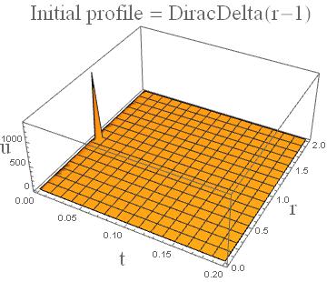
----- Initial profile = DiracDelta peak at r = 1

The r integral gives immediately

adelta[k_, R_] = k R^(5/4) BesselJ[1/4, k R];

and the solution is (the exact integral is not performed by MMA)

udelta[r_, t_, R_] := 
 NIntegrate[
  adelta[k, R] Exp[-3 k^2 t] BesselJ[1/4, k r]/r^(1/4), {k, 0, \[Infinity]}]

Here is the plot

Plot3D[udelta[r, t, 1], {t, 0, 0.2}, {r, 0, 2}, 
  AxesLabel -> {Text[Style["t", Large]], Text[Style["r", Large]], 
    Text[Style["u", Large]]}, 
  PlotLabel -> Text[Style["Initial profile = DiracDelta(r-1)", Large]],  
  PlotRange -> All] // Quiet

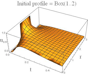
----- Initial profile = box (= 1 für 1<r<2)

aa1[k_] = k Integrate[ r^(5/4) BesselJ[1/4, k r], {r, 1, 2}]

(* Out[61]= -BesselJ[5/4, k] + 2 2^(1/4) BesselJ[5/4, 2 k] *)

ubox[r_, t_] := 
 NIntegrate[
  aa1[k] Exp[-3 k^2 t] BesselJ[1/4, k r] /r^(1/4), {k, 0, \[Infinity]}]


Plot3D[ubox[r, t], {t, 0, .5}, {r, 0, 3}, 
  AxesLabel -> {Text[Style["t", Large]], Text[Style["r", Large]], 
    Text[Style["u", Large]]}, 
  PlotLabel -> Text[Style["Initial profile = Box(1..2)", Large]],  
  PlotRange -> All] // Quiet

Section 2.2: given functions $a(k)$

----- Example 1: a = 1

us1[x_, t_] = 
 Integrate[ Exp[-3 k^2 t] BesselJ[1/4, k r] /r^(1/4), {k, 0, \[Infinity]}, 
  Assumptions -> {t > 0, r > 0}]

(*
Out[210]= (E^(-(r^2/(24 t))) Sqrt[\[Pi]] BesselI[1/8, r^2/(24 t)])/(2 Sqrt[3] r^(
 1/4) Sqrt[t])
*)

You can look at the plot (not shown here)

Plot3D[us1[r, t], {r, 0, 4}, {t, 0, 1}]

----- Example 2: a[k] = DiracDelta[k-1]

giving

us2[r_, t_] := Exp[-3 t] BesselJ[1/4, r ] /r^(1/4)

Plot3D[us2[r, t], {r, 0, 20}, {t, 0, 1}, PlotRange -> All] (* not shown here *)