2
$\begingroup$

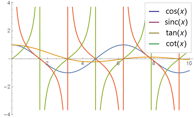
I am using the below code to create legends but I don't know why the colors in legends for various plots are different of devoted to main color of plots

From http://reference.wolfram.com/language/ref/Inset.html?q=Inset in Application part:

legendPlot[xl_List, d_, args___] := 
 Plot[xl, d, 
 Epilog -> 
 Inset[Panel[
 Grid[MapIndexed[{Graphics[{ColorData[1, First@#2], Thick, 
       Line[{{0, 0}, {1, 0}}]}, AspectRatio -> .5, 
      ImageSize -> 20], #1} &, xl]]], 
  Offset[{-2, -2}, Scaled[{1, 1}]], {Right, Top}], args]
 legendPlot[{Cos[x], Sinc[x], Tan[x], Cot[x]}, {x, 0, 10}]

Sinc is Orange in the main plot Tan is Green, Cot is Red!!!!

enter image description here

$\endgroup$
3
  • 1
    $\begingroup$ What version are you using? That looks like Mathematica's newer default colors on the plot and the old default colors on the legend! $\endgroup$
    – march
    Commented Nov 29, 2015 at 4:40
  • $\begingroup$ Looks like the legendPlot is using older version for colors. The first workaround would be defining a new color code and using that color code at both plots. $\endgroup$
    – gurluk
    Commented Nov 29, 2015 at 4:47
  • $\begingroup$ I am using version 10 both plot and legend!! $\endgroup$ Commented Nov 29, 2015 at 4:58

2 Answers 2

5
$\begingroup$

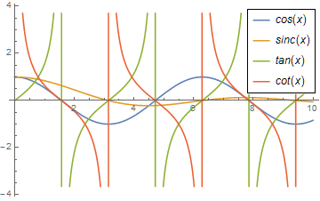
As an alternative implementation, consider

frame[legend_] := Framed[legend, FrameStyle -> Black, RoundingRadius -> 0, 
    FrameMargins -> 0, Background -> White];
legendPlot[xl_List, d_] := Plot[xl, d, PlotLegends -> Placed[LineLegend[
    "Expressions", LabelStyle -> Italic, LegendFunction -> frame], {.88, .75}]];
legendPlot[{Cos[x], Sinc[x], Tan[x], Cot[x]}, {x, 0, 10}]

enter image description here

To answer the specific question, the colors in the Plot and Epilog of the Question are different, because the colors used by Plot are not ColorData[1, ...]. Replace 1 by 97 for better agreement. The complete list of indexed colors can be displayed with

MatrixForm[Table[{i, ColorData[i, "ColorList"]}, {i, ColorData["Indexed"]}], 
    TableAlignments -> Left]
$\endgroup$
2
$\begingroup$

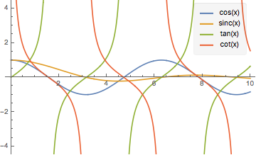
Adding in exclusions, just for interest.

plot = Plot[{Cos[x], Sinc[x], Tan[x], Cot[x]}, {x, 0, 10}];

colourpositions = Position[plot, _RGBColor, Infinity];

colours = Extract[plot, colourpositions];

tanplot = Plot[Tan[x], {x, 0, 10},
   Exclusions -> Map[Pi #/2 &, 2 Range[10] - 1],
   PlotStyle -> colours[[3]]];

cotplot = Plot[Cot[x], {x, 0, 10},
   Exclusions -> Map[Pi #/2 &, 2 Range[10]],
   PlotStyle -> colours[[4]]];

otherplots = Plot[{Cos[x], Sinc[x]}, {x, 0, 10}];

Show[otherplots, tanplot, cotplot,
 PlotRange -> {Automatic, {-4, 4}},
 Epilog -> Inset[Panel[Grid[MapThread[
      {Graphics[{#2, Thick, Line[{{0, 0}, {1, 0}}]},
         AspectRatio -> 0.5, ImageSize -> 20], #1} &,
      {Through[{Cos, Sinc, Tan, Cot}@"x"], colours}]]],
   Offset[{-12, -2}, Scaled[{1, 1}]], {Right, Top}]]

enter image description here

$\endgroup$
1
  • $\begingroup$ It's very good because the vertical lines of (Tan and Cot) are removed and there is a interval of manual picking of colors $\endgroup$ Commented Nov 29, 2015 at 13:24

Your Answer

By clicking “Post Your Answer”, you agree to our terms of service and acknowledge you have read our privacy policy.

Not the answer you're looking for? Browse other questions tagged or ask your own question.