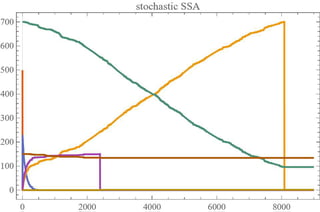
1
$\begingroup$

I want to apply the Gillespie algorithm to a set of reactions. First, I run the source code presented here, and then run my model:

ClearAll[a, b, c, d, e, f, g, h, t];
reactions = {a -> Null, a -> b, b -> c, b -> d, c + e -> 2 c, 
d + f -> 2 d, 700 c -> g, c + g -> g, 150 d -> h, d + h -> h};
vars = {a, b, c, d, e, f, g, h};
rates = {0.5, 0.5, 0.004, 0.006, 0.000000595, 0.000000411, 1000, 1000,
1000, 1000};
init = <|a -> 500, b -> 0, c -> 0, d -> 0, e -> 700, f -> 150, g -> 0,
h -> 0|>;
sto = GillespieSSA[reactions, init, rates, {0, 2.5*3600}];
op = {PlotStyle -> Thick, PlotTheme -> "Scientific"};
Plot[Evaluate@Through@sto@t, {t, 0, 2.5*3600}, Evaluate@op, 
PlotLabel -> "stochastic SSA", PlotLegends -> Automatic, PlotRange -> Full]
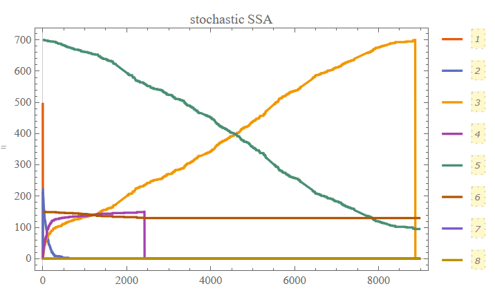
enter image description here

I need to verify this result using other approaches to code Gillespie algorithm. I found a package here which says it can implement Gillespie algorithm, but I cannot figure it out how to apply it to my model above. Any help is appreciated!

$\endgroup$
6
  • $\begingroup$ I was wondering what happened to the purple guys around $t=2400$ and the yellow guys around $t=8000$, but then I noticed the 700 c -> g and 150 d -> h reactions. It seems like these reactions occur very quickly after c hits 700 and d hits 150. Is this what you want? $\endgroup$
    – Chris K
    Commented May 14 at 18:37
  • $\begingroup$ Sorry, I've only used @IstvánZachar's function (with a few tweaks to the syntax I made). If this is a chemical reaction network, I think 700 c -> g would indicate an event when 700 c's ran into each other to react and form one g. Doesn't seem right to me, but you know your problem better. Perhaps you could add a description of the system you're modeling? $\endgroup$
    – Chris K
    Commented May 14 at 18:49
  • $\begingroup$ @Anovice How we can interpreter Null in your reactions? $\endgroup$ Commented May 20 at 12:19
  • $\begingroup$ @Anovice Unfortunately in paclet you try to use Null treated as a variable Null[t] :) $\endgroup$ Commented May 20 at 13:16
  • $\begingroup$ @Anovice Maybe we can use it as variable null to make model? $\endgroup$ Commented May 20 at 14:34

1 Answer 1

2
+250
$\begingroup$

It is not complete answer since paclet we try to use has some typos in it (maybe it needs just version update). At first step we compute data using GillespieSSA code above with a fixed random generator state

SeedRandom[1234];

As result we have

plot1=Plot[Evaluate@Through@sto@t, {t, 0, 2.5*3600}, Evaluate@op, 
PlotLabel -> "stochastic SSA", PlotLegends -> Automatic, PlotRange -> Full] 

Figure 1

Now we install paclet (use this line only once)

PacletInstall["RobertNachbar/CompartmentalModeling"]

After installation complete we call

Needs["RobertNachbar`CompartmentalModeling`"]

Now we can use paclet as follows

reactions = {a -> null, a -> b, b -> c, b -> d, c + e -> 2 c, 
   d + f -> 2 d, 700 c -> g, c + g -> g, 150 d -> h, d + h -> h};
vars = {a, b, c, d, e, f, g, h};
rates = {0.5, 0.5, 0.004, 0.006, 0.000000595, 0.000000411, 1000, 1000,
    1000, 1000};
init = <|a -> 500, b -> 0, c -> 0, d -> 0, e -> 700, f -> 150, g -> 0,
    h -> 0|>;

model = Table[
  Transition[reactions[[i, 1]], rates[[i]], reactions[[i, 2]]], {i, 
   Length[reactions]}]
vars0 = {a0, b0, c0, d0, e0, f0, g0, h0}; params = 
 Table[vars0[[i]] -> init[vars[[i]]], {i, Length[vars0]}]
modelData = 
 PacletSymbol[
  "RobertNachbar/CompartmentalModeling", 
   "RobertNachbar`CompartmentalModeling`KineticCompartmentalModel"][
  model, t]
state = Replace[modelData["Variables"], 
  Join[Thread[vars -> vars0], {_ -> 0}], {1}]; SeedRandom[1234];

sol =
 PacletSymbol[
  "RobertNachbar/CompartmentalModeling", 
   "RobertNachbar`CompartmentalModeling`StochasticSolve"][
  modelData["Rates"] /. params, 
  modelData["StoichiometricMatrix"] // Normal, state /. params, 
  modelData["Variables"], {t, 0, 2.5*3600}]

There are several messages concerning data interpolation, and we have out mixed data where c,d are not interpolated. It is why we use

 lstc = Evaluate[c /. sol[[1]]][[1]]; lstd = 
 Evaluate[d /. sol[[1]]][[1]]; 

Finally we compare two models

Show[plot1,Plot[Evaluate[{a@t, b@t, e@t, f@t, g@t, h@t} /. sol[[1]]], {t, 0, 
   2.5  3600}, PlotStyle -> Dashed, PlotRange -> All], 
 ListPlot[{lstc, lstd}, PlotStyle -> {Green, Magenta}, PlotLegends -> {c, d}]]
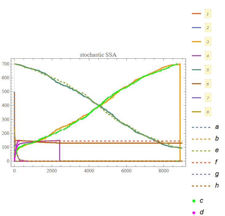
Figure 2

$\endgroup$
4
  • 1
    $\begingroup$ @Anovice Yes, you are right. I add more legends. $\endgroup$ Commented May 20 at 16:40
  • 1
    $\begingroup$ @Anovice Actually we have sol that consists of data ready to plot. We can plot data together or separate, with triangles or with any other PlotMarkers. $\endgroup$ Commented May 22 at 14:52
  • 1
    $\begingroup$ @Anovice We can use Table[Plot[sto[[i]]@t, {t, 0, 2.5*3600}, PlotLabel -> vars[[i]], PlotLegends -> Automatic, PlotRange -> All], {i, Length[vars]}] to plot vars separately, or, for example, Plot[sto[[1]]@t, {t, 0, 2.5*3600}, PlotLabel -> vars[[1]], PlotLegends -> Automatic, PlotRange -> All] to plot a only. $\endgroup$ Commented May 22 at 17:40
  • 1
    $\begingroup$ @Anovice Please, pay attention that Out for a looks like a-> InterpolatingFunction[..], and for c -> Interpolation[...]. Rule a->InterpolatingFunction is ready to use, but for c we need to extract data first. $\endgroup$ Commented May 22 at 18:41

Your Answer

By clicking “Post Your Answer”, you agree to our terms of service and acknowledge you have read our privacy policy.