15
$\begingroup$

I try to solve a nonlinear integro-differential equation with this code. Here i used a periodic condition.

L=10; tmax = 2;

NDSolve[{D[u[x, t], t] + u[x, t]*D[u[x, t], x] + D[u[x, t], {x, 2}] + 
D[u[x, t], {x, 4}] + 1/(2 L)*NIntegrate[D[u[xp, t],{xp, 3}]*Cot[\[Pi](x - xp)/(2*L)], {xp, -L, x, L}, Method -> {"PrincipalValue"}] == 0,
u[-L, t] == u[L, t], u[x, 0] == 0.1*Cos[\[Pi]/L*x]}, u, {x, -L, L}, {t, 0, tmax}]

which gives me

NDSolve::delpde:Delay partial differential equations are not currently supported by NDSolve"

The warning is understandable because the function u[xp, t] is still unknow when NIntegrate is evaluated. Note that we should use PrincipalValue here in NIntegrate because there is a singularity at $x=xp$, which has been specified in the integration range.

$\endgroup$
13
  • $\begingroup$ The method I used to solve the earlier problem cited in the question cannot be employed here, because the PDE is nonlinear. It may, however, be possible to solve the equation using the method outlined here, although not without a great deal of effort. $\endgroup$
    – bbgodfrey
    Commented Feb 24, 2019 at 20:08
  • $\begingroup$ My answer to question 175080 may be helpful, although it is a bit simpler. $\endgroup$
    – bbgodfrey
    Commented Feb 25, 2019 at 5:13
  • $\begingroup$ If you solve this problem, please post your solution as an answer. $\endgroup$
    – bbgodfrey
    Commented Feb 25, 2019 at 23:13
  • $\begingroup$ Perhaps, I can try near the end of the week, if you have not already done so. $\endgroup$
    – bbgodfrey
    Commented Feb 26, 2019 at 4:26
  • $\begingroup$ I think it would be advisable to change the order of D[NIntegrate[...]] to NIntegrate[D[...]]. This would mean replacing D[Integrate[u[xp, t]*Cot[\[Pi] (x - xp)/(2*L)], {xp, -L, L}], {x, 3}] with NIntegrate[-((\[Pi]^3 (2 + Cos[(\[Pi] (x - xp))/L]) Csc[(\[Pi] (x - xp))/(2 L)]^4 u[xp, t])/(4 L^3)), {xp, -L, L}], where the integrand in the second form was found with D[u[xp, t]*Cot[\[Pi] (x - xp)/(2*L)], {x, 3}] // FullSimplify. $\endgroup$
    – Roman
    Commented Feb 26, 2019 at 13:31

3 Answers 3

10
$\begingroup$

Based on the hacky way I used in my answer here; I had to split up the NDSolve process, so as not to redefine MapThread too soon:

L = 10; tmax = 2;
sys = {D[u[x, t], t] + u[x, t]*D[u[x, t], x] + D[u[x, t], {x, 2}] + 
     D[u[x, t], {x, 4}] + 1/(2 L)*int[D[u[x, t], {x, 3}], x, t] == 0, 
   u[-L, t] == u[L, t], u[x, 0] == 0.1*Cos[\[Pi]/L*x]};
periodize[data_] := Append[data, {N@L, data[[1, 2]]}]; (* for periodic interpolation *)
Block[{int},
  (* the integral *)
  int[uppp_, x_?NumericQ, t_ /; t == 0] := (cnt++;
    NIntegrate[
     D[0.1*Cos[\[Pi]/L*xp], {xp, 3}]*Cot[\[Pi] (x - xp)/(2*L)],
     {xp, x - L, x, x + L}, 
     Method -> {"InterpolationPointsSubdivision", Method -> "PrincipalValue"},
     PrecisionGoal -> 8, MaxRecursion -> 20, AccuracyGoal -> 20]);
  int[uppp_?VectorQ, xv_?VectorQ, t_] := Function[x,
     cnt++;
     NIntegrate[
      Interpolation[periodize@Transpose@{xv, uppp}, xp, 
        PeriodicInterpolation -> True]*Cot[\[Pi] (x - xp)/(2*L)],
      {xp, x - L, x, x + L}, 
      Method -> {"InterpolationPointsSubdivision", Method -> "PrincipalValue"},
      PrecisionGoal -> 8, MaxRecursion -> 20] (* adjust to suit *)
     ] /@ xv;
  (* monitor while integrating pde *)
  Clear[foo];
  cnt = 0;
  PrintTemporary@Dynamic@{foo, cnt, Clock[Infinity]};
  (* broken down NDSolve call *)
  Internal`InheritedBlock[{MapThread},
   {state} = NDSolve`ProcessEquations[sys, u, {x, -L, L}, {t, 0, tmax}, 
     StepMonitor :> (foo = t)];
   Unprotect[MapThread];
   MapThread[f_, data_, 1] /; ! FreeQ[f, int] := f @@ data;
   Protect[MapThread];
   NDSolve`Iterate[state, {0, tmax}];
   sol = NDSolve`ProcessSolutions[state]
   ]] // AbsoluteTiming

enter image description here

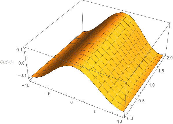
Plot3D[u[x, t] /. sol, {x, -10.`, 10.`}, {t, 0.`, 2.`}]

enter image description here

With the settings PrecisionGoal -> 4, MaxRecursion -> 9 in the NIntegrate, it takes the same amount of time and does more integrations. Breaking down the NDSolve process is explained in the tutorial Components and Data Structures.

$\endgroup$
17
  • 1
    $\begingroup$ Very impressive (+1). Thanks. $\endgroup$
    – bbgodfrey
    Commented Mar 6, 2019 at 17:21
  • $\begingroup$ @Michael E2, your method is cool and far outside of my knowledge range about mma. Could you explain a little the reason Method -> {"InterpolationPointsSubdivision", Method... } in NIntegrate. I quickly go through tutorial/NIntegrateIntegrationStrategies, and found the general specification NIntegrate[f[x],{x,a,b,c}, Method->{"PrincipalValue",Method->methodspec,"SingularPointIntegrationRadius"->\[Epsilon]}], which appears to be different from yours. Thank you for your answer. $\endgroup$
    – user55777
    Commented Mar 7, 2019 at 4:04
  • $\begingroup$ By testing the code as it is, i encounter the usual warning: >NIntegrate::slwcon: Numerical integration converging too slowly; suspect one of the following: singularity, value of the integration is 0, highly oscillatory integrand, or WorkingPrecision too small. I don't understand the issue because the singular point has been specified. Please give me suggestion. Thanks a lot. $\endgroup$
    – user55777
    Commented Mar 7, 2019 at 4:34
  • 2
    $\begingroup$ @user55777 Some posts concerning "InterpolationPointsSubdivision" shows use-cases, but it's not well documented. Basically, interpolating functions have (weak) singularities at the interpolation points (nodes), and integration rules are more effective on intervals over which functions do not have singularities. By dividing up the interval of integration at the interpolation points, convergence is more easily obtained. It can be inefficient if there are a lot of interpolation points. $\endgroup$
    – Michael E2
    Commented Mar 7, 2019 at 19:31
  • 1
    $\begingroup$ Technically, it is a preprocessor "strategy" and so can take another Method argument, which may be another "strategy" or "rule." See NIntegrate Introduction, Strategies, Rules, and Preprocessors $\endgroup$
    – Michael E2
    Commented Mar 7, 2019 at 19:35
4
$\begingroup$

After studying during these days, now I could answer the question myself. I admit that both my solution and code are far from good and efficient, even some mistakes or making an unnecessary move. Please give your suggestion if you see anything.

We first create $2M$ equidistant grid points $x_m=(m-M)h$ with $m=1,2,...,2M$. The x-position of the grid points is stored in xtab:

M = 40; L = 10; h = L/M;
xtab = Table[(m - M) h, {m, 1, 2*M}];

Then we should discretize the solution of PDE along $x$ into $2M$ solutions of a set of coupled ODEs. u[m][t] denotes the solution of function $u(x,t)$ at point $x_m$. Here, I didn't include the left end-point, since it can be set to be u[0][t]=u[2*M][t] according to the periodicity.

U[t_] = Table[u[m][t], {m, 1, 2*M}];

The spatial derivatives are discretized using 2nd-order central differences, here the periodic condition should be applied. Because I didn't know how to generate these derivatives using ListCorrelate both for boundary points and internal points in one-line command, I manually add the derivatives near the boundary. Please give me some advice if you know how to do this.

1st-derivative wrt x:

internaldUdx = ListCorrelate[{-1, 0, 1}/(2 h), U[t]]; (* for 2<= m <= 19*)
dUdx = Join[{(u[2][t] - u[2*M][t])/(2 h)}, 
internaldUdx, {(u[1][t] - u[2*M - 1][t])/(2 h)}];

2nd-derivative wrt x:

internaldUdxx = ListCorrelate[{1, -2, 1}/h^2, U[t]]; (* for 2<= m<=19 *)
dUdxx = Join[{(u[2][t] - 2*u[1][t] + u[2*M][t])/h^2}, 
internaldUdxx, {(u[1][t] - 2 u[2*M][t] + u[2*M - 1][t])/h^2}];

3rd-derivative wrt x

internaldUdxxx = ListCorrelate[{-1, 2, 0, -2, 1}/(2 h^3), U[t]]; (*for 3<= m <= 2*M-2*)
dUdxxx = Join[{(-u[2 M - 1][t] + 2 u[2 M][t] - 2 u[2][t] + u[3][t])/(2 h^3), (-u[2*M][t] + 2 u[1][t] - 2 u[3][t] + u[4][t])/(2 h^3)}, 
internaldUdxxx, {(-u[2*M - 1 - 2][t] + 2*u[2*M - 1 - 1][t] - 2*u[2*M - 1 + 1][t] + u[1][t])/(2 h^3), (-u[2*M - 2][t] + 2 u[2*M - 1][t] - 2 u[1][t] + u[2][t])/(2 h^3)}];

4th-derivative wrt x:

internaldUdxxxx = ListCorrelate[{1, -4, 6, -4, 1}/h^4, U[t]]; (*for 3 <= m <= 2M-2*)
dUdxxxx = Join[{(u[2*M - 1][t] - 4*u[2*M][t] + 6*u[1][t] - 4*u[1 + 1][t] + 
 u[1 + 2][t])/h^4, (u[2*M][t] - 4*u[1][t] + 6*u[2][t] - 4*u[2 + 1][t] + u[2 + 2][t])/h^4}, 
internaldUdxxxx, {(u[2*M - 3][t] - 4*u[2*M - 2][t] + 6*u[2*M - 1][t] - 4*u[2*M][t] + u[1][t])/h^4, (u[2*M - 2][t] - 4*u[2*M - 1][t] + 6*u[2*M][t] - 4 u[1][t] + u[2][t])/h^4}];

To discretize the integral, we may introduce the mid-points: $x_{m+1/2}=(x_m+x_{m+1})/2$ for $m=1,2,....,2M-1$ with $x_{1/2}=(-L+x_1)/2$.

midxtab = Join[{(-L + (1 - M) h)/2}, Table[((m - M) h + (m + 1 - M) h)/2, {m, 1, 2*M - 1}]];
int[midP_] := h/(2 L)*dUdxxxIntP.Cot[\[Pi]*(midxtab[[midP]] - xtab)/(2*L)]

Constructing the system of ODEs and the discrete initial condition:

eqns = Thread[D[U[t], t] == -U[t]*dUdx - dUdxx - dUdxxxx - 
 Join[Table[1/2*(int[midP] + int[midP + 1]), {midP, 1, 2*M - 1}], {int[2*M] + int[1]}]];

initc = Thread[U[0] == 1/10*Cos[\[Pi]/L*xtab]];

The original PDE now can be solved numerically:

tmax = 10;

lines = NDSolveValue[{eqns, initc}, U[t], {t, 0, tmax},
Method -> {"EquationSimplification" -> "Solve"}] // Flatten;

Then, we can plot by interpolating (appreciating @bbgodfrey's answer to a related question)

surf = Flatten[Table[{(line - M)*h, t, lines[[line]]}, {line, 1, 2*M}, {t, 0, 
 tmax, 0.2}], 1];

ListPlot3D[surf, PlotRange -> All, AxesLabel -> {"x", "t", "u"}, ImageSize -> Large, LabelStyle -> {Black, Bold, Medium}]
$\endgroup$
2
  • $\begingroup$ You did not use PrincipalValue, although you indicated that you should use. $\endgroup$ Commented Mar 6, 2019 at 13:11
  • $\begingroup$ Parameter is not defined dUdxxxIntP. $\endgroup$ Commented Mar 6, 2019 at 16:13
3
$\begingroup$

We can use iterations. The code is simple but takes time.

L = 10; tmax = 2; del = 10^-6; dx = (L - del)/6 - del;
n = 5;
int[0][x_, t_] := 0
Do[U[i] = 
  NDSolveValue[{D[u[x, t], t] + u[x, t]*D[u[x, t], x] + 
      D[u[x, t], {x, 2}] + D[u[x, t], {x, 4}] + 
      1/(2 L)*int[i - 1][x, t] == 0, u[-L, t] == u[L, t], 
    u[x, 0] == 0.1*Cos[\[Pi]/L*x]}, u, {x, -L, L}, {t, 0, tmax}, 
   Method -> {"PDEDiscretization" -> {"MethodOfLines", 
       "SpatialDiscretization" -> {"TensorProductGrid", 
         "MinPoints" -> 137}}}]; 
 int[i] = Interpolation[
   Flatten[ParallelTable[{{x, t}, 
      NIntegrate[
       Derivative[3, 0][U[i]][xp, t]*
        Cot[\[Pi] (x - xp)/(2*L)], {xp, -L, x, L}, 
       Method -> "PrincipalValue"]}, {x, -L + del, L - del, dx}, {t, 
      0, tmax, .2*tmax}], 1]];, {i, 1, n}]


Table[Plot3D[U[i][x, t], {x, -L, L}, {t, 0, tmax}], {i, 1, n}]
Table[Plot3D[
  int[i][x, t] - int[i - 1][x, t], {x, -L, L}, {t, 0, tmax}, 
  PlotRange -> All], {i, 1, n}]

fig1

$\endgroup$
3
  • $\begingroup$ thank you. I found that with the same conditions, your code is much faster than Michael's. Could I consult you three questions: 1. what determine the choice of n = 5? I consider it as an iterator for the calculation of integral, but didn't see a convergence criterion; 2. you actually use FD in x?; 3. Does Table[Plot3D[U[i][x, t], {x, -L, L}, {t, 0, tmax}], {i, 1, n}] only give the intermediate solutions. But how can i plot a convergent u[x,t] with something like Plot3D[u[x, t]/.finalsol, {x, -L, L}, {t, 0, tmax}]? $\endgroup$
    – user55777
    Commented Mar 7, 2019 at 14:58
  • $\begingroup$ U[i][x, t] this is a solution to the equation at each iteration i. The final solution of the equation U[n][x, t] depends on the selected error. $\endgroup$ Commented Mar 7, 2019 at 16:17
  • $\begingroup$ In this example, only convergence is shown. You can add a line of code outside the loop using int[n][x, t] to calculate finalsol. $\endgroup$ Commented Mar 8, 2019 at 12:00

Your Answer

By clicking “Post Your Answer”, you agree to our terms of service and acknowledge you have read our privacy policy.

Not the answer you're looking for? Browse other questions tagged or ask your own question.