3
$\begingroup$

I already asked a question regarding how to solve a nonlinear pde in mathematica which was answered nicely.

https://mathematica.stackexchange.com/questions/134145/solving-a-non-linear-pde

Actually this was a 1-dimensional form of a general 2D problem that I was trying to solve with matlab, but first I wanted to have a clue about the solution using mathematica. Now I think I have to restrict myself into solving it in mathematica. Here is the 2D form of the problem with its initial and boundary conditions:

$$\frac{\partial h}{\partial t} = -0.01 \bigg(\frac{\partial}{\partial x}\Big(h^3 \big(\frac{\partial^3h}{\partial x^3}+\frac{\partial ^3h}{\partial x\partial y^2}\big)\Big)+ \frac{\partial }{\partial y}\Big(h^3 \big(\frac{\partial ^3h}{\partial y^3}+\frac{\partial ^3h}{\partial y\partial x^2}\big)\Big)\bigg)$$ $$\frac{\partial h}{\partial x}=0,\ \ \frac{\partial^3h}{\partial x^3}+\frac{\partial ^3h}{\partial x\partial y^2}=0\ \ \text{when}\ \ x=\pm1$$ $$\frac{\partial h}{\partial y}=0,\ \ \frac{\partial ^3h}{\partial y^3}+\frac{\partial ^3h}{\partial y\partial x^2}=0\ \ \text{when}\ \ y=\pm1$$ $$h(0,x,y)=1+\cos(\pi x) \cos(\pi y)$$ I tried to do the same as the 1D case, however it gives me an error with the boundary conditions. I tried this:

t0 = 6;
BCLx1 = Derivative[0, 1, 0][u][t, -1, y];

BCRx1 = Derivative[0, 1, 0][u][t, 1, y];

BCLx3 = Derivative[0, 3, 0][u][t, x, -1]+Derivative[0, 1, 2][u][t, -1, y];

BCRx3 = Derivative[0, 3, 0][u][t, x, 1]+Derivative[0, 1, 2][u][t, 1, y];

BCLy1 = Derivative[0, 0, 1][u][t, x, -1];

BCRy1 = Derivative[0, 0, 1][u][t, x, 1];

BCLy3 = Derivative[0, 0, 3][u][t, x, -1]+Derivative[0, 2, 1][u][t, x, -1];

BCRy3 = Derivative[0, 0, 3][u][t, x, 1]+Derivative[0, 2, 1][u][t, x, 1];

sol = NDSolve[{D[u[t, x, y], 
 t] == -0.0192*
               (D[u[t, x, y]^3*(D[u[t, x, y], {x, 3}] + 
                D[D[u[t, x, y], {y, 2}], x]), x] + 
                D[u[t, x, y]^3*(D[u[t, x, y], {y, 3}] + 
                D[D[u[t, x, y], {x, 2}], y]), y]), 
          u[0, x, y] == Cos[π y] Cos[π x] + 1,
          BCLx1 == 0, 
          BCRx1 == 0, 
          BCLx3 == 0, 
          BCRx3 == 0, 
          BCLy1 == 0, 
          BCRy1 == 0, 
          BCLy3 == 0, 
          BCRy3 == 0}, 
      u, {t, 0, t0}, {x, -1, 1}, {y, -1, 1}, Method -> {"MethodOfLines", 
"SpatialDiscretization" -> {"TensorProductGrid", "MinPoints" -> 100}}, 
PrecisionGoal -> 2]; Plot3D[{u[t0, x, y] /. sol}, {y, -1, 1}, {x, -1, 1}, PlotRange -> All]

It states that the boundary conditions include non-normal derivatives! but they are all meaningful BCs based on the physics of the problem.

Any help in this regard is highly appreciated.

$\endgroup$
3
  • 1
    $\begingroup$ Your translation for BCRx3 and BCLx3 is wrong. Still, NDSolve isn't able to handle these b.c.s even after correcting this. Are you sure the b.c.s are correct? What material are you referring to? $\endgroup$
    – xzczd
    Commented Dec 27, 2016 at 5:24
  • $\begingroup$ This problem represents the leveling of a liquid film over a flat surface as a function of time. These two papers address this problem in a more general way (which is not the case for me and I have made it simpler without any unrealistic change): $\endgroup$ Commented Dec 27, 2016 at 10:18
  • 1
    $\begingroup$ The problem represents the leveling of a liquid film on a flat surface as a function of time. These two papers address this problem in a general way (which is not the case for me; I have made it simpler without any unrealistic change): 1-Numerical simulation of thin paint film flow, Bruno Figliuzzi eta al, 2012 2-Three-Dimensional Direct Numerical Simulation of Surface-Tension-Gradient Effects on the Leveling of an Evaporating Multicomponent Fluid, M. H. Eres, 1998 Based on the problem, the slope(dh/dx) and the flux (qx =d^3h/dx^3+d^3h/dxdy^2) of the liquid at the boundaries are all zero. $\endgroup$ Commented Dec 27, 2016 at 10:23

1 Answer 1

3
$\begingroup$

OK, even after the incorrect translation for BCRx3 and BCLx3 is amended, NDSolve can't handle this kind of boundary conditions, so let's discretize spatial dimensions outside of NDSolve, with the help of pdetoode:

t0 = 6;
BCLx1 = Derivative[0, 1, 0][u][t, -1, y];
BCRx1 = Derivative[0, 1, 0][u][t, 1, y];
BCLx3 = Derivative[0, 3, 0][u][t, -1, y] + Derivative[0, 1, 2][u][t, -1, y];
BCRx3 = Derivative[0, 3, 0][u][t, 1, y] + Derivative[0, 1, 2][u][t, 1, y];
BCLy1 = Derivative[0, 0, 1][u][t, x, -1];
BCRy1 = Derivative[0, 0, 1][u][t, x, 1];
BCLy3 = Derivative[0, 0, 3][u][t, x, -1] + Derivative[0, 2, 1][u][t, x, -1];
BCRy3 = Derivative[0, 0, 3][u][t, x, 1] + Derivative[0, 2, 1][u][t, x, 1];
eqn = D[u[t, x, y], 
    t] == -0.0192*(D[u[t, x, y]^3*(D[u[t, x, y], {x, 3}] + D[D[u[t, x, y], {y, 2}], x]), 
       x] + D[u[t, x, y]^3*(D[u[t, x, y], {y, 3}] + D[D[u[t, x, y], {x, 2}], y]), y]);
ic = u[0, x, y] == Cos[π y] Cos[π x] + 1;
bc = {BCLx1 == 0, BCRx1 == 0, BCLx3 == 0, BCRx3 == 0, BCLy1 == 0, BCRy1 == 0, BCLy3 == 0,
    BCRy3 == 0};

xdomain = ydomain = {-1, 1};
xpoints = ypoints = 30;
xgrid = Array[# &, xpoints, xdomain];
ygrid = Array[# &, ypoints, ydomain];
difforder = 4;
var = Outer[u, xgrid, ygrid];
(* Definition of pdetoode isn't included in this code piece, 
   please find it in the link above. *)
ptoo = pdetoode[u[t, x, y], t, {xgrid, ygrid}, difforder];

del = Delete[#, {{1}, {2}, {-2}, {-1}}] &;
ode = del /@ del@ptoo@eqn;
odeic = del /@ del@ptoo@ic;
odebc = MapAt[del, ptoo@bc, List /@ Range@4];

sollst = NDSolveValue[{ode, odeic, odebc}, var, {t, 0, t0}, 
                      SolveDelayed -> True]; // AbsoluteTiming
(* {8.970609, Null} *)

sol = rebuild[sollst, {xgrid, ygrid}, -1];

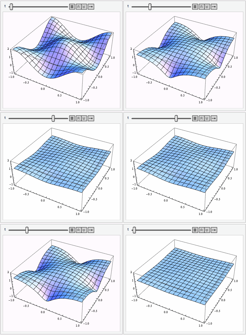
Animate[
 Plot3D[sol[x, y, t], {x, xdomain} // Flatten // Evaluate, {y, ydomain} // Flatten // 
   Evaluate, PlotRange -> {-1, 2}, PerformanceGoal -> "Quality"], {t, 0, 1/2}]

enter image description here

SolveDelayed -> True option is necessary at least for v10.2, its color is red, but don't worry.

$\endgroup$
20
  • $\begingroup$ I copy and paste this code with pdetoode dosen't work! $\endgroup$ Commented Dec 27, 2016 at 12:05
  • $\begingroup$ @MariuszIwaniuk As mentioned above, the definition of pdetoode isn't included in this post, please find it in the link at the beginning of the post. $\endgroup$
    – xzczd
    Commented Dec 27, 2016 at 12:07
  • $\begingroup$ i'm add a pdetoode code.I.have error messages: \!\({t, 0, 6}[\"ValuesOnGrid\"]\) cannot be used as a variable. $\endgroup$ Commented Dec 27, 2016 at 12:09
  • $\begingroup$ @MariuszIwaniuk Show me a screen shot? $\endgroup$
    – xzczd
    Commented Dec 27, 2016 at 12:14
  • 1
    $\begingroup$ @S.Cho Which version are you in? Anyway, if you just need a workaround, try e.g. lst = Table[ Plot3D[sol[t, x, y], {x, xdomain} // Flatten // Evaluate, {y, ydomain} // Flatten // Evaluate, PlotRange -> {-1, 2}], {t, 0, 1/2, 1/48}]; ListAnimate@lst $\endgroup$
    – xzczd
    Commented Jan 30, 2019 at 16:14

Your Answer

By clicking “Post Your Answer”, you agree to our terms of service and acknowledge you have read our privacy policy.

Not the answer you're looking for? Browse other questions tagged or ask your own question.