This small note describes the method I use. I've been using this method for years. (all of my web site is written in Latex actually, and converted to HTML. First I used to use latex2html then switched to tex4ht few years ago as it is better supported and it comes with texlive).
To use Mathematica to generate HTML, the idea is to mix Latex inside the notebook, and generate the computation result to latex file on the fly as the program runs.
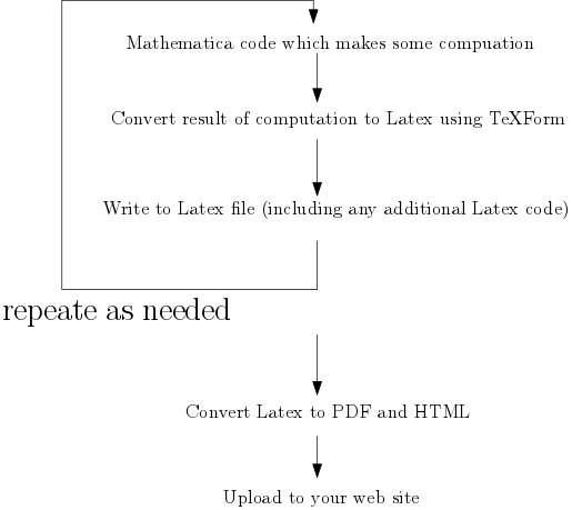
This method have many advantages, but it requires one to know some Latex to use it.
It uses Latex as the gateway between CAS and HTML. CAS generates Latex, tex4ht converts Latex to HTML. pdflatex converts Latex to PDF.
There are mainly two method to mix CAS generated computation with Latex.
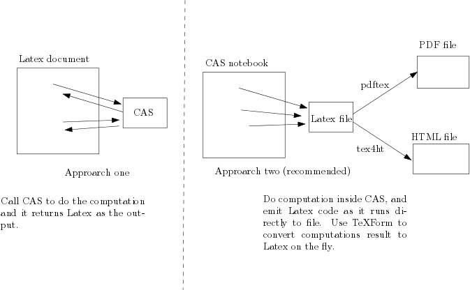
The first method is what packages such as pythontex uses. The second method is what I think is the better method. It is more robust.
Advantages of generating Latex from Mathematica (instead of say HTML) are many:
First, one gets a PDF file for free along the way. This is huge advantage.
Second, one gets all the features that comes with Latex/tex4ht, such as automatic table of contents generation (with HTML links to other pages), automatic href link generation from inside the document, breaking large document into many smaller HTML pages and having all the HTML links automatically generated, automatic bibliography generated to HTML, And many more. (try to do all this with manual HTML coding :)
So Mathematica is used only to generate Latex. TeXForm is used heavily in this process. The rest is done by tex4ht and pdflatex if one wants pdf file as well.
I use this method all the time. As an example, I just generated this 300 pages document by a program I wrote in Mathematica over one week time, which Shows the step by step solution of simple 1st order ODE's from textbooks. Converted to HTML pages with tex4ht.
To illustrate this method, I used the example posted here.
To do this easily, CODE input cell is better suited for this than INPUT cell (since lots of Latex code is used inside the notebook, it is easier to format using CODE cell)
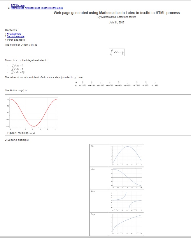
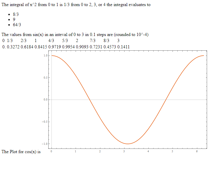
I'll post the code used. Here is a link to HTML page generated and the PDF file as well and the notebook I used. (will add small screen shot below as well)
Here is the code listing as well (same as in the above link) (this can be improved more, it was done quickly. This actually builds everything into one string. But in actual reports, I send Latex output to file immediately).
SetDirectory[NotebookDirectory[]];
ClearAll[x,s];
tex[s_] := ToString@TeXForm[s];

fileName ="index.tex";
file=OpenWrite[fileName,PageWidth->Infinity];

from=0; to=1;
int=HoldForm[Integrate[x^2,{x,0,1}]];

s="
\\documentclass[11pt]{article}
\\usepackage{amsmath}
\\usepackage{graphicx}
\\usepackage{array}
\\usepackage[letterpaper,  margin=1in]{geometry}
\\usepackage{longtable}
\\usepackage{float}
\\usepackage{hyperref}
\\begin{document}

\\ifdefined\\HCode
\\href{index.pdf}{PDF file here}
\\href{example_making_web_page.nb}{Mathematica notebook used to generate the Latex}
\\fi

\\title{Web page generated using Mathematica to Latex to tex4ht to HTML process}
\\date{\\today}
\\author{By Mathematica, Latex and tex4ht}
\\maketitle
\\tableofcontents
\\section{First example}
   The integral of $x^2$ from $"<>tex[from]<>"$ to $"<>tex[to]<>"$ is
   \\[
      \\boxed{ " <>tex[int]<>" = "<> tex[ReleaseHold[int]]<>"}
   \\]
   From $0$ to $2 \\dots 4$ the integral evaluates to
   \\begin{itemize}
";

  Do[
     With[{n=i},
          int=HoldForm@Integrate[x^2,{x,0,n}];
          s=s<>"\\item $"<>tex[int]<>" = "<> tex[ReleaseHold@int] <>"$\n"
     ]
    , {i,2,4}
  ];
  s=s<>"\\end{itemize}
  The values of $\\sin(x)$ in an inteval of $0$ to $3$ in $0.1$ steps (rounded to $10^{-4}$ are
  \\["<>
  tex[TableForm@Transpose@Table[{x,N@Round[Sin[x],10^-4]},{x,0,3,1/3}]]<>
  "\\]
  The Plot for $\\cos(x)$ is";
  p=Plot[Cos[x], {x, 0, 2 Pi},Frame->True,PlotStyle->Red,GridLines->Automatic,GridLinesStyle->LightGray];
  Export["myImage.pdf",p];
  s=s<>"
     \\begin{figure}[H]
     \\centering
        \\includegraphics[width=0.5\\textwidth]{myImage}
     \\caption{my plot of $\\cos(x)$}
     \\end{figure}
  ";

s=s<>"
     \\section{Second example}\n";
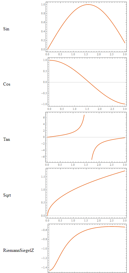
     functions = {Sin, Cos, Tan, Sqrt, RiemannSiegelZ}
     s=s<>"\\begin{center}
           %\\begin{table}
           \\begin{longtable}{|l|m{.7\\textwidth}|}\\hline \n";
     Do[
         s=s<>"$"<>tex[functions[[i]]]<>"$&";
         p=Plot[functions[[i]][x], {x, 0, 3},Frame->True,ImagePadding->20,GridLines->Automatic,GridLinesStyle->LightGray];
         imageName = "myImage"<>ToString[i]<>".pdf";
         Export[imageName,p];
         imageName = "myImage"<>ToString[i];
         s=s<>"\\includegraphics[width=0.3\\textwidth]{"<>imageName<>"}\\\\ \\hline \n"
         ,
        {i, 1, Length@functions}
     ];
     s=s<>"\\end{longtable}
           %\\caption{My table of functions}
           %\\end{table}
           \\end{center}";
     s=s<>"\\end{document}";
     WriteString[file,s];
     Close[file];
Running the above generates index.tex in the same folder. This file is then compiled using the command make4ht index.tex which generated the HTML pages.




StartProcessis too). Theme development actually took longer, because I'm not a web programmer. $\endgroup$