I was trying to plot the residual for the solution of my PDE. However, I was unsure about a couple of things.
I imported the data and created an Interpolation polynomial with
ListInterpolationI am trying to replace the dependant variable
hin my equation with the interpolation polynomial,solutionusingreplaceor/.I would need to plot this equation for different/consecutive steps in time to see what the residual looks like. (
residual = equation(t) - equation(t-1))
Either all this or is there any way I could just generate the residual from some magic mathematica function?
Should I be defining something as a function of time, which is one of the arguments (? is this the right word) in the interpolating function polynomial?
The notebook and data files are attached for anyone's convenience.
I can't seem to put my finger on the problem but I can't plot the residuals. I apologize if the question is sophomoric but I can't seem to master mathematica at all like other programming environments.
Minimum working example:
Equation solver (script file)
#!/usr/local/bin/MathematicaScript -script

$HistoryLength=0;
$pwf=$InputFileName;
Needs["VectorAnalysis`"]
Needs["DifferentialEquations`InterpolatingFunctionAnatomy`"];
Clear[Eq0,EvapThickFilm,h,Bo,ϵ,K1,δ,Bi,m,r]
Eq0[h_,{Bo_,ϵ_,K1_,δ_,Bi_,m_,r_}]:=\!\(
\*SubscriptBox[\(∂\), \(t\)]h\)+Div[-h^3 Bo Grad[h]+h^3 Grad[Laplacian[h]]+(δ h^3)/(Bi h+K1)^3 Grad[h]+m (h/(K1+Bi h))^2 Grad[h]]+ϵ/(Bi h+K1) + (r)D[D[(h^2/(K1+Bi h)),x] h^3,x] ==0;
SetCoordinates[Cartesian[x,y,z]];
EvapThickFilm[Bo_,ϵ_,K1_,δ_,Bi_,m_,r_]:=Eq0[h[x,y,t],{Bo,ϵ,K1,δ,Bi,m,r}];
TraditionalForm[EvapThickFilm[Bo,ϵ,K1,δ,Bi,m,r]];


L=79.5788; TMax=12500*100;
Off[NDSolve::mxsst];
Clear[Kvar];
Kvar[t_]:=  Piecewise[{{1,t<=1},{2,t>1}}]
(*Ktemp = Array[0.001+0.001#^2&,13]*)
hSol=h/.NDSolve[{
(*Bo,ϵ,K1,δ,Bi,m,r*)

EvapThickFilm[0,1*10^-6,1,0.001,1,2*0.025,0],
h[0,y,t]==h[L,y,t],
h[x,0,t]==h[x,L,t],
(*h[x,y,0] == 1.1+Cos[x] Sin[2y] *)
h[x,y,0]==1+(-0.05 Cos[2π x/L] -0.05 Sin[2 π x/L])(Cos[2π y/L])
},
h,
{x, 0, L},
{y,0, L},
{t, 0, TMax},
Method->{"LSODA","MaxDifferenceOrder"->12},
MaxStepFraction->1/50,
PrecisionGoal->3
][[1]]


{TMin,TRup}=InterpolatingFunctionDomain[hSol][[3]];
hSolGridData=InterpolatingFunctionValuesOnGrid[hSol];
hSolCoords=InterpolatingFunctionCoordinates[hSol];
finalStep=InterpolatingFunctionCoordinates[hSol][[3]];
(*rupture=NumberForm[N[TRup/100],6];*)
rupture=TRup/100;

$parameterfile=StringJoin[$pwf,".dat"];
Export[$parameterfile, {0, 100, 0, 0.0001, 35.1, 7.02, 0, 3, 1, 5, SetPrecision[rupture,5]}];
$matfile=StringJoin[$pwf,".mat"];
Export[$matfile,hSolGridData];
(*Exports time step data*)
$timefile=StringJoin[$pwf,"_time",".mat"];
Export[$timefile,InterpolatingFunctionCoordinates[hSol][[3]]];

hGrid = InterpolatingFunctionGrid[hSol];
{TMin,TRup}=InterpolatingFunctionDomain[hSol][[3]];
Length[hGrid];
{nX,nY,nT}=Drop[Dimensions[hGrid],-1];

fac=0.98;


$epsfile0=StringJoin[$pwf,"_0",".eps"];
$pngfile0=StringJoin[$pwf,"_0",".png"];
$epsfileRup=StringJoin[$pwf,"_TRup",".eps"];
$pngfileRup=StringJoin[$pwf,"_TRup",".png"];
ic=Plot3D[hSol[x,y,0*TRup],{x,0,L},{y, 0, L},

PlotRange->{{0,L},{0,L},{0,3.5}},
BaseStyle->{FontWeight->"Plain",FontSize->18},
PlotPoints->65,
ColorFunction->GrayLevel
];
Export[$epsfile0,ic,ImageSize->{350,350}];
Export[$pngfile0,ic,ImageResolution->350];
rupProfile=Plot3D[hSol[x,y,fac*TRup],{x,0,L},{y, 0, L},

PlotRange->{{0,L},{0,L},{0,3.5}},
BaseStyle->{FontWeight->"Plain",FontSize->18},
PlotPoints->65,
ColorFunction->GrayLevel
];
Export[$epsfileRup,rupProfile,ImageSize->{350,350}];
Export[$pngfileRup,rupProfile,ImageResolution->350];

dataxy=Import[$matfile];
datat=Import[$timefile];


(*$epsfile0=StringJoin[$pwf,"_0_dft",".eps"];
$pngfile0=StringJoin[$pwf,"_0_dft",".png"];
$epsfileRup=StringJoin[$pwf,"_TRup_dft",".eps"];
$pngfileRup=StringJoin[$pwf,"_TRup_dft",".png"];
FDataFirst=Abs[Fourier[dataxy[[All,All,1]]]];
dftfirst=MatrixPlot[FDataFirst]*)
Data collection where I try to "replace" dependant variable with inter. polynomial
$HistoryLength = 0;
Needs["VectorAnalysis`"]
Needs["DifferentialEquations`InterpolatingFunctionAnatomy`"];
L = 79.5788;
dataxy = Import[
   "/home/dnaneet/Desktop/residuals/L_lambda_max_1wl_zg_E_0001_Cos.\
mat"];
datat = Import[
   "/home/dnaneet/Desktop/residuals/L_lambda_max_1wl_zg_E_0001_Cos_\
time.mat"];
solution = ListInterpolation[dataxy, {{0, L}, {0, L}, Flatten[datat]}];
trup = Max[Flatten[datat]]
tsrup = Ceiling[
   0.95 Flatten[Position[Ceiling[Flatten[datat]], Ceiling[trup]]]];
ts = tsrup[[1]];

Clear[Eq0, FilmEqn, h, Bo, ϵ, K1, δ, Bi, m, r]
Eq0[h_, {Bo_, ϵ_, K1_, δ_, Bi_, m_, r_}] := \!\(
\*SubscriptBox[\(∂\), \(t\)]h\) +
   Div[-h^3 Bo Grad[h] +
     h^3 Grad[Laplacian[h]] + (δ h^3)/(Bi h + K1)^3 Grad[h] +
     m (h/(K1 + Bi h))^2 Grad[h]] + ϵ/(
   Bi h + K1) + (r) D[D[(h^2/(K1 + Bi h)), x] h^3, x] /.
  h -> solution[All, All, xtime]
SetCoordinates[Cartesian[x, y, z]];
FilmEqn[Bo_, ϵ_, K1_, δ_, Bi_, m_, r_] :=
  Eq0[h[x, y, t], {Bo, ϵ, K1, δ, Bi, m, r}];

TraditionalForm[
 FilmEqn[0, 10^-6, 1, 10^-3, 1, 0.05,
  0]](*Eqn=Simplify[FilmEqn[0,10^-6,1,10^-3,1,0.05,0]];*)
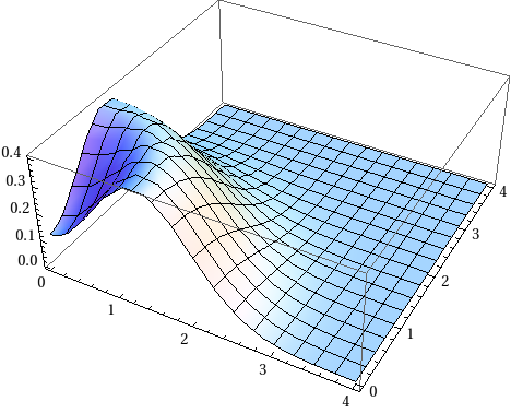
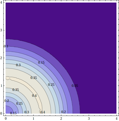
The film plot should look like this:
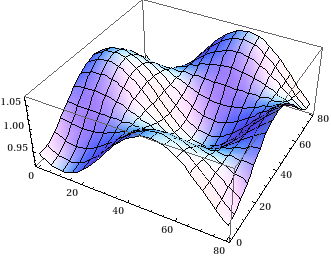
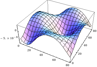
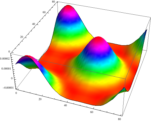
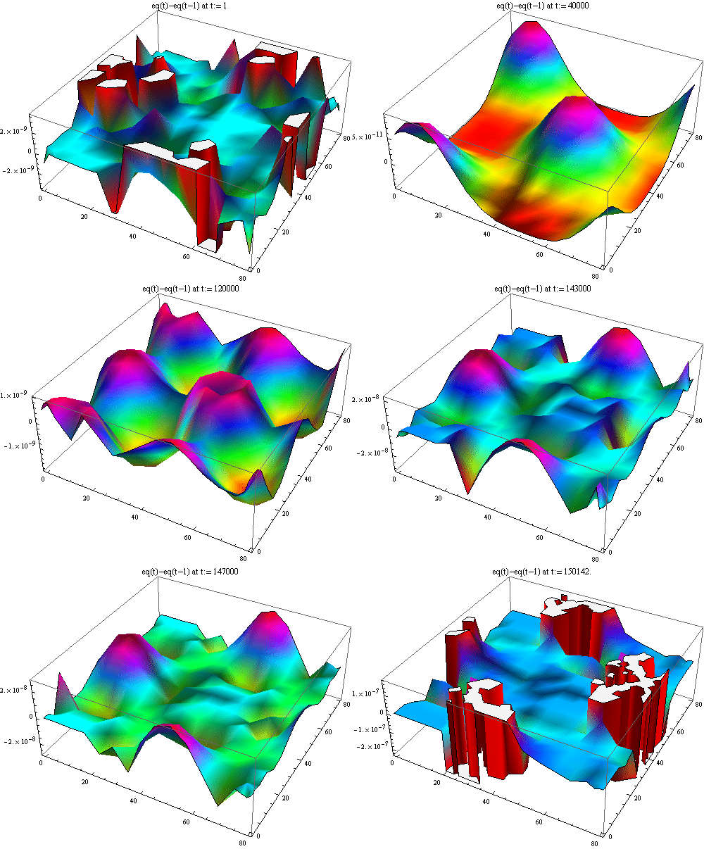
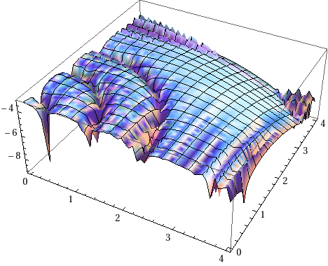
My interpretation of the residual Any thoughts or comments?
Plot3D[
 solution[x, y, 100000] - solution[x, y, 99999],
 {x, 0, L},
 {y, 0, L}
 ]

ListInterpolation, sample-data, equation, ... which can all be shown with a small example which can be completely included here. Meaning, I don't have to download a notebook, because you post all code here and create random example data. The dropbox thing will not live forever and later, people cannot not take advantage of your question and the answers because it is incomplete. $\endgroup$solution[All, All, 1000]is no list access and if you intended it like this, then you probably express the thing you want in a wrong way. $\endgroup$