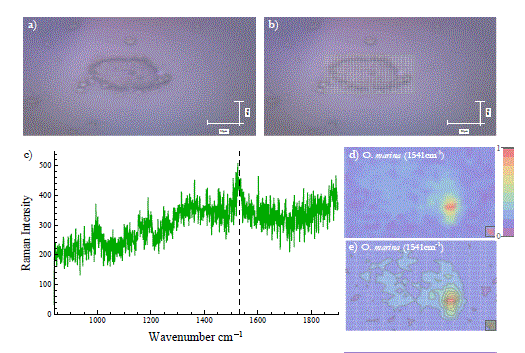
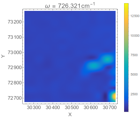
The first thing you need to do is to extract the x and y value from the filename, that's what the StringCases is doing below. Then you want to import the data from the text files and prepend the x and y values to each element of the spectrum, that's what the Join is doing.
filenamelist = FileNames["*.txt"];
import[fn_] :=
 Join[Flatten@
     ToExpression@
      StringCases[fn,
       "X_" ~~ a__ ~~ "__Y_" ~~ b__ ~~ "__Time" -> {a, b}], #] & /@
  Import[fn, "Table"]
data = Flatten[import /@ filenamelist, 1];
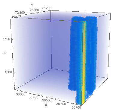
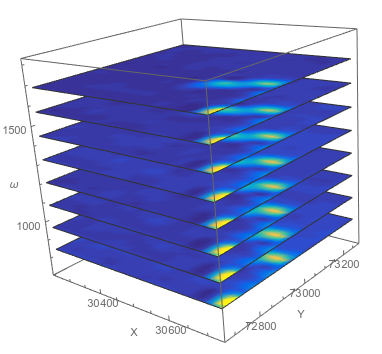
You can plot the entire data set at once using one of the 4-dimensional plotting functions, like ListDensityPlot3D or ListSliceDensityPlot3D
<< "http://pastebin.com/raw.php?i=sqYFdrkY"(*This imports my favorite color function :-)  *)
ListDensityPlot3D[data,
 ColorFunction -> ParulaCM, AxesLabel -> {"X", "Y", "ω"}]

ListSliceDensityPlot3D[data, {"ZStackedPlanes", 8},
 ColorFunction -> ParulaCM, AxesLabel -> {"X", "Y", "ω"}]

But these 4-dimensional plots (x, y, omega, and color) are hard to view information from, so I like to use 2D density plots personally. So let's split the data up into different lists for each frequency,
dataSR = GatherBy[data, #[[3]] &][[All,
   All, {1, 2, 4}]];(*the spectrally-resolved raman maps*)
frequencies =
 DeleteDuplicates[data[[All, 3]]]; (* a list of the frequencies *)
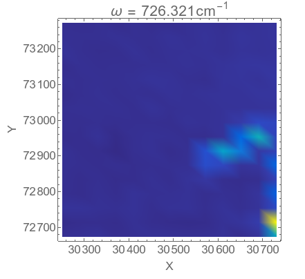
Now we can make a density plot for a single frequency,
ListDensityPlot[dataSR[[1]], ColorFunction -> ParulaCM,
 PlotRange -> All, PlotLabel ->
  Row[{"\[Omega] = ", frequencies[[1]],
    "\!\(\*SuperscriptBox[\(cm\), \(-1\)]\)"}],
 FrameLabel -> {"X", "Y"}, BaseStyle -> 16, ImageSize -> 400]

You notice that it is a bit blocky, and that is due to the fact that the spatial resolution is low. There are only 16 grid points in the x direction and 13 in the y direction.
You can interpolate the data to get a better plot if you like, but to do so you need to reshape the data into the form of an array,
{xrange, yrange, \[Omega]range, intensityrange} =
  MinMax /@ Transpose[data];
ListDensityPlot[Transpose@Partition[dataSR[[1, All, 3]], 16],
 ColorFunction -> ParulaCM, PlotRange -> All, InterpolationOrder -> 2,
  PlotLegends -> Automatic,
 PlotLabel ->
  Row[{"\[Omega] = ", frequencies[[1]],
    "\!\(\*SuperscriptBox[\(cm\), \(-1\)]\)"}],
 FrameLabel -> {"X", "Y"}, BaseStyle -> 16, ImageSize -> 400,
 DataRange -> {xrange, yrange}]

I think that looks pretty decent, but you may prefer the non-interpolated form as an honest display of the data, up to you. You could also change the plotting scale, perhaps using a nonlinear scale to highlight weak features, or omit the PlotRange->All option so that the bright spot in the corner doesn't override the plot.
You can do a density plot for all the different frequencies and collect them in an image list,
imglist =
  ListDensityPlot[Transpose@Partition[dataSR[[#, All, 3]], 16],
     ColorFunction -> ParulaCM, PlotRange -> All,
     InterpolationOrder -> 2, PlotLegends -> Automatic,
     PlotLabel ->
      Row[{"\[Omega] = ", frequencies[[#]],
        "\!\(\*SuperscriptBox[\(cm\), \(-1\)]\)"}],
     FrameLabel -> {"X", "Y"}, BaseStyle -> 16, ImageSize -> 400,
     DataRange -> {xrange, yrange}] & /@ Range[Length@frequencies];
which can then be exported as a movie file, or you can scan through it manually using Manipulate
Manipulate[imglist[[n]], {{n, 1}, 1, Length@imglist, 1}]

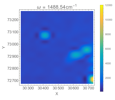
As you can see from the movie, there isn't a lot of variation of the map with different frequencies, there are mostly just the three bright spots, but if you scan more slowly you can find interesting bits like this

Hope this helps.

