NSolve for high degree univariate polynomials

Question

I am trying to solve a high degree univariate polynomial using Mathematica's NSolve command. But when I plug the solutions generated by Mathematica back to the equations, the equations are massive numbers and not even close to zero.

Clear["Global`*"];
r := Rationalize[RandomReal[NormalDistribution[0, 1]]]
randompol[n_, i_] := Sum[r Sqrt[Binomial[n, j]] x^j, {j, 0, n}]

e= randompol[100,1];

SetSystemOptions["NSolveOptions" -> {"Tolerance" -> 10^(-10)}];
sol = Solve[e == 0, x];

e/.sol

which gives some of the entries as big as -1.8513*10^56

I don't know what other method can be used to solve high degree polynomials. Any help would be much appreciated. Regards, -John

Answer 1

I did a few things:

(1) Set the second argument of Rationalize to a definite, but arbitrary, value so that exact numbers (fractions) were produced by Rationalize. Your original code did not give exact numbers for r.

(2) Forced the coefficients of the polynomial to have high precision.

(3) Dropped the second argument of randompol . Deleted the SetSystemsOptions.

(4) Set a high Working Precision -> 200 within NSolve.

Clear["Global`*"];

r := Rationalize[RandomReal[NormalDistribution[0, 1]], 0.001]


randompol[n_] := 

Sum[r SetPrecision[Sqrt[Binomial[n, j]], 1000] x^j, {j, 0, n}] 


e = randompol[100];

sol = NSolve[e == 0, x, WorkingPrecision -> 200]; 

Abs[e /. sol] // Max

(* 0.*10^-103 *)

Which indicates that e is much closer to zero than when I used your original code. I was suspicious of such quick and easy success, but a look at the sol values themselves suggests that they are indeed very high precision numbers.

sol[[1]]

{x -> -6.0238372136976606502260060478459892247764184751597217356329032\

6202362152948359151728116621315272069788936311451308262538189004899677\

26114562119851606529164803119604073806915565538453032032195787093638 \

- 1.520416566625392687364937426390455945886297726051920478299290947504\

9036377745161941667006869410482430785120127207233197413002926845477907\

689127706303421233595275524517422427858590001778013216673664575 I}

P.S. Yes, I considered a different problem than the one you posed, in order to introduce a level of discreteness to the polynomial coefficients. If you evaluate:

r := Rationalize[s = RandomReal[NormalDistribution[0, 1]]]
{r, s, r - s, Precision[r], Precision[s], Precision[r - s]}

(*  {-0.203065, -0.203065, 0., MachinePrecision, MachinePrecision,  *)
(*    MachinePrecision}                                             *)

you can see that Rationalize, without a second argument, doesn't do anything to a machine number as its first argument; the result is just a machine number, not a rational. So, rationals were not being produced in your original code.

The documentation of Rationalize seems to suggest that the smallest value for its second argument is 0. In that case, the denominators of the rationals produced by Rationalize seem to have 9 decimal digits, at most, in which case setting WorkingPrecision->200 in NSolve will produce the kind of good agreement for Abs[e /. sol] // Max shown earlier. With 0 as the second argument of Rationalize, the SetPrecision[ . . . ,1000] I inserted into the Sum expression of your original code was unnecessary. This would have been more a more direct code response:

r := Rationalize[RandomReal[NormalDistribution[0, 1]], 0]
randompol[n_] := Sum[r Sqrt[Binomial[n, j]] x^j, {j, 0, n}] 
e = randompol[100];
sol = NSolve[e == 0, x, WorkingPrecision -> 200];
Abs[e /. sol] // Max
(*  0.*10^-21  *)

Thank you for commenting on my original answer.

Answer 2

NSolve works fine

Basically, there is nothing wrong with the result that Solve/NSolve produces, or at least the errors are slight. The number 10^166 may not seem that close to zero, but that depends on whether it is compared with 1 or 10^175. Since NSolve solves for x, the best you can hope for is that all the bits in the machine number for x are correct. In practice, the last few bits may be wrong due to round-off error in computing function values.

On SetPrecision[.., Infinity] and epsilon

Let me review a few facts about machine floating-point numbers that I wish to refer to in my explanation. A (binary) machine real x is a rational number of the form x0 = mantissa * 2^exponent, where mantissa is represented with a fixed number of bits. Changing the lowest-order bit corresponds to changing x by the smallest amount ϵ possible. The real number x can be thought of as representing a real number that lies between x0 ± ϵ/2, with a maximum uncertainty of ϵ/2; the point-estimate x0 is the number used in computation. In a computational process there can be round-off error that gets propagated resulting in a number x that has a uncertainty greater than ϵ/2. In Mathematica, the ϵ for the number x = 1 is given by $MachineEpsilon (on my machine, $MachineEpsilon == 2.220446049250313*^-16 == 2^(-52)). For a number x, one can estimate the corresponding ϵ with $MachineEpsilon * x. One can get the exact number x0 with x0 = SetPrecision[x, Infinity].

Two Three explanations

There are two three ways to explain why e /. x -> sol[[1]] can result in a number larger than 10^166 when sol[[1]] gives the best possible approximation of the root (at machine precision). For the sake of reproducibility, here is the code I used from the OP, with a slight change (Rationalize did nothing on the coefficients generated):

SeedRandom[1];
(*r := Rationalize[RandomReal[NormalDistribution[0,1]]];*)
r := RandomReal[NormalDistribution[0, 1]];
e = randompol[100, 1];
sol = NSolve[e == 0, x];

Update: Using Solve

If we use Solve on the exact equation, we can check these solutions against the ones returned by NSolve. The equation has to have exact coefficients or Solve uses numerical techniques.

solexact = Solve[SetPrecision[e, Infinity] == 0, x];

(x /. sol) == Sort@N[x /. solexact]
Sort@N[x /. solexact] - (x /. sol) // Abs // Max
(*
  True
  3.55271*10^-15
*)

Here we see Solve did in fact return solutions (of course!).

ParallelMap[FullSimplify, 
  SetPrecision[e, Infinity] /. solexact] // AbsoluteTiming
(*
  {77.192719, {0, 0, 0, 0, 0, 0, 0, 0, 0, 0, 0, 0, 0, 0, 0, 0, 0, 0, 0, 0, 0, 0,
     0, 0, 0, 0, 0, 0, 0, 0, 0, 0, 0, 0, 0, 0, 0, 0, 0, 0, 0, 0, 0, 0, 0, 0, 0, 
     0, 0, 0, 0, 0, 0, 0, 0, 0, 0, 0, 0, 0, 0, 0, 0, 0, 0, 0, 0, 0, 0, 0, 0, 0, 
     0, 0, 0, 0, 0, 0, 0, 0, 0, 0, 0, 0, 0, 0, 0, 0, 0, 0, 0, 0, 0, 0, 0, 0, 0, 
     0, 0, 0}}
*)

Perhaps the answer should stop here. Originally I was interested in explaining the numerics because this issue has come up before. I thought having an explanation of why NSolve appears to have done a bad job but in fact did a good job might be helpful.

The propagation of the error in x in the value of the polynomial

First, if y = f[x], then for a given error dx in x, the corresponding error dy in y is approximated by

dy = f'[x] dx

The size of dy evidently depends on the size of f'[x]. Let us take sol[[1]] as an example (it produces the greatest value of e). If dx is on the order of 0.5 $MachineEpsilon * x and the derivative D[e, x] /. sol[[1]] of the OP's equation is on the order of 10^180, then dy will be on the order of

Abs[D[e, x] (0.5 $MachineEpsilon*x)] /. sol[[1]]
(*
  1.77676*10^166
*)

The magnitude of e, which is the error from 0, is about twice that,

e /. sol[[1]]
(*
  -3.82848*10^166
*)

suggesting either round-off error in the calculation of e or error in the result of NSolve. If the error is due to NSolve, the error is not much since the uncertainty in x appears to be a little more than $MachineEpsilon * x. It appears that the root in sol[[1]] might be off in its last binary bit from what is optimal. In any case, it's a good-looking result.

Precision and round-off error in evaluating the polynomial

But not so fast. A second way to analyze the situation is as follows. Mathematica can track precision, if so-called arbitrary-precision numbers are used. We can turn precision-tracking on, by setting the precision to $MachinePrecision.

SetPrecision[e, $MachinePrecision] /. SetPrecision[sol[[1]], $MachinePrecision]
Accuracy[%]
(*
  0.*10^168
  -168.799
*)

Mathematica is indicating that the result is 0 within an error less than about ±10^168. Our original value -3.8*^166 for e /. sol[[1]] is well within that error. What is happening is a tremendous loss of precision in computing e /. sol[[1]]. If we set the precision high enough, we can calculate the value of e at the (exact rational) number computed for sol[[1]].

SetPrecision[e, 50] /. SetPrecision[sol[[1]], 50];
Precision[%]     (* check precision *)
N[%%]            (* print as a machine Real *)
(*
  31.3568
  -1.28981*10^166
*)

By controlling the round-off error in calculating e, we see that the value for e is within the estimated maximum error 1.77676 * 10^166. This suggests that the computed value for x is the best possible. We can check that with the number within ±ϵ. They give values of e further from zero:

With[{eps = SetPrecision[$MachineEpsilon, 50], 
  sol = SetPrecision[sol[[1]], 50]},
 {SetPrecision[e, 50] /. x -> (x - eps x /. sol),
  SetPrecision[e, 50] /. x -> (x + eps x /. sol)} // N
 ]
(*
  {-4.84333*10^166, 2.2637*10^166}
*)

Thus we see that NSolve actually computed the best approximation to the real root for the case sol[[1]].

On the accuracy of the solutions

With the other roots, it is more or less the same, that (1) the computed number for x is the best or nearly best possible approximation of the root and (2) the value of e is due to a round-off error and/or a large value of D[e, x]. About half give the best possible solution. In most other cases, the error is in the last one or two bits, but that might not be surprising given the sort of numerical difficulty e presents. The worst cases are the complex conjugate pair sol[[{57, 58}]] which are 12 ϵ away from the best exact solution (as found by FindRoot Solve). Below we see the value of e is less at x - 12 eps;

SetPrecision[e, 50] /. SetPrecision[sol[[57]], 50] // Abs // N
With[{eps = 2^Floor@Log2@Abs[$MachineEpsilon Re[x]] /. sol[[57]]},
   SetPrecision[e, 50] /. 
    x -> (x - 12 eps /. SetPrecision[sol[[57]], 50])
   ] // Abs // N
(*
  1.25526*10^46
  2.91146*10^45
*)

The code below finds how far each solution found by NSolve is from each root (measured in relative epsilons).

dxeps = MapThread[
  Function[{x, xexact}, 
   Through[{Re, Im}[(xexact) - (x)]] / 
      {2^Floor@Log2@Abs[$MachineEpsilon Re[x0]], 
       2^Floor@Log2@Abs[$MachineEpsilon Im[x0]]} /. x0 -> x
   ],
  {x /. sol, Sort@N[x /. solexact]}
  ]

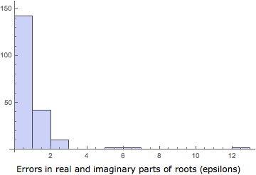
48 of 100 solutions are best possible; the worst cases are solutions 57/58.

Count[dxeps, {0., 0.}]
(*
  48
*)

Position[#, Max@#] &@ Abs @ dxeps
(*
  {{57, 1}, {58, 1}}
*)

Distribution of errors:

Labeled[
 Histogram[Flatten @ Abs @ dxeps],
 Style["Errors in real and imaginary parts of roots (epsilons)", "Label"]
 ]

Getting more accurate results

Update: Perhaps one should just use Solve as above. I'll leave the explanation below because I find it interesting, even if it's rather useless in this case.

As mentioned by user15996, to get solutions that produce values for e that are zero to some number of digits of accuracy, greater working precision is needed. First, we will need to set the precision of the coefficients of the polynomial e to be exact (or of sufficient precision), which I'll call eP. As an example let's consider sol[[57]]. We see below that there is a deficit of almost 49 digits, that is, Mathematica is telling us that the value is zero with an error less than 10^49. So if we use a WorkingPrecision of 49 digits plus $MachinePrecision, we should end up with an accuracy around 0 digits. It's a little tricky to get exactly 0 because the real and imaginary parts have different accuracies. We can increase the WorkingPrecision to get a positive number of significant digtis.

eP = SetPrecision[e, Infinity];

eP /. SetPrecision[sol[[57]], $MachinePrecision]
accuracydeficit = Max[-Accuracy /@ {Re[%], Im[%]}]
(*
  0``-48.9342823110845 + 0``-48.95998064695299 I
  48.96
*)

extraprecision = 0;
extraprecision + accuracydeficit + $MachinePrecision
solWP = NSolve[eP == 0, x, 
   WorkingPrecision -> extraprecision + accuracydeficit + $MachinePrecision];
eP /. solWP[[57]]
(*
  64.9146
  0``0.025698335868500944 + 0``0 I
*)

extraprecision = 2;
solWP = NSolve[eP == 0, x, 
   WorkingPrecision -> extraprecision + accuracydeficit + $MachinePrecision];
eP /. solWP[[57]]
(*
  0``2.025698335868505 + 0``2. I
*)

The value of the polynomial with MachinePrecision coefficients is still way off, for the same reasons as before, round-off error with insufficient precision.

e /. solWP[[57]]
(*
  -3.37129*10^45 - 2.92341*10^45 I
*)

Therefore to get solutions that will evaluate eP to $MachinePrecision accurately, we should pick the maximum accuracy deficit:

accuracydeficit = 
 Max[-Map[Accuracy, 
          Through[{Re, Im}[eP /. SetPrecision[sol, $MachinePrecision]]],
          {-1}]]
extraprecision = $MachinePrecision;
extraprecision + accuracydeficit + $MachinePrecision
solWP = NSolve[eP == 0, x, 
   WorkingPrecision -> extraprecision + accuracydeficit + $MachinePrecision];
(*
  168.795
  200.704
*)

Check solWP (this returns the result with the lowest accuracy):

Through[{Re, Im}[eP /. solWP]] // Max
(*
  0.*10^-16
*)