Caveat: the technique below seems to fail for matrices as large as the OP wants, and I'm not sure why. See the last paragraph.
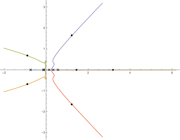
The eigenvalues are the roots of the characteristic polynomial of the matrix; and buried deep within Mathematica is a method to create a plot of the roots of a polynomial as a function of a parameter
d = 6;
samplemat = DiagonalMatrix[RandomReal[{-1, 1}, d]] + a RandomReal[{-1, 1}, {d, d}];
polynom[x_] = CharacteristicPolynomial[samplemat, x];
RootLocusPlot[1/polynom[x], {a, 0, 5}, FeedbackType -> None, ImageSize -> Large]

The crosses are the initial locations of the roots (a = 0 in this case); the lines are the paths of the roots in the complex plane as a goes from 0 to 5. By default, the dots are placed at the locations of the roots when the parameter is halfway from its maximum to its minimum (a = 2.5 in this case.)
A tip of the hat to this previous answerthis previous answer, which is where I learned of this functionality.
That said: this method starts throwing errors for d = 8 and higher, which means that this method wouldn't work for a $14 \times 14$ matrix. These errors seem to be internal to the RootLocusPlot function (they're generated by functions like Transpose, Part, and MapThread), and I don't know enough about this function specifically or control functions in general to try to diagnose it. I'm posting this answer all the same, in the hopes that someone who knows more about the inner workings of Mathematica than I do will be able to refine my answer, and because this technique might still be useful to a future Googler with a smaller matrix and/or less complicated matrix.
