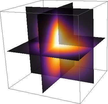
My preferred method for this kind of thing is projecting each dimension onto a plane and then combining them together. I think MATLAB has similar functionality. Mind you, the answers and comments on my question about projecting are right in pointing out that this will become inefficient for high polygon counts (essentially more PlotPoints) so if you want to Manipulate in a smooth way, you may want to use Texture. See this relevant question for details on that.

Now, I haven't got your function psi1XYsq so I will pick a double gaussian:

E^(-(x^2 + (y - 2)^2 + (z - 3)^2)/10) + E^(-((x + 1)^2 + (y + 2)^2 + (z + 2)^2)/25)

The idea is to use something similar to the function @Jens is using in his answer to How to make a drop-shadow for a Graphics3D objects?.

Block[{d1, d2, d3, function, options, opacity, x0, y0, z0, min, max},
 {min, max} = {-9, 9};
 {x0, y0, z0} = {0., 0., 0.};
 opacity = 0.9;
 function[x_, y_, z_] := 
  E^(-(x^2 + (y - 2)^2 + (z - 3)^2)/10) + 
   E^(-((x + 1)^2 + (y + 2)^2 + (z + 2)^2)/25);
 options = Sequence @@ {PlotPoints -> 45, Mesh -> None, 
    ColorFunctionScaling -> False, ColorFunction -> "SunsetColors"};
 d1 = First@DensityPlot[function[x, y, z0], {x, min, max}, {y, min, max}, 
     Evaluate@options] /. {x_?AtomQ, y_?AtomQ} -> {x, y, z0};
 d2 = First@DensityPlot[function[x, y0, z], {x, min, max}, {z, min, max}, 
     Evaluate@options] /. {x_?AtomQ, z_?AtomQ} -> {x, y0, z};
 d3 = First@DensityPlot[function[x0, y, z], {y, min, max}, {z, min, max}, 
     Evaluate@options] /. {y_?AtomQ, z_?AtomQ} -> {x0, y, z};
 Show[Graphics3D[{d1, d2, d3}, Lighting -> "Neutral"] /. 
   GraphicsComplex[xx__] -> {Opacity[opacity], GraphicsComplex[xx]}]
 ]

The code is straightforward: min, max define the range for each variable, {x0, y0, z0} define the projection planes, and opacity the Opacity. You will notice I have turned off ColorFunctionScaling so that each slice is bright according to an absolute value and they merge together nicely. If your function is not normalised you may want to normalise it before doing that.

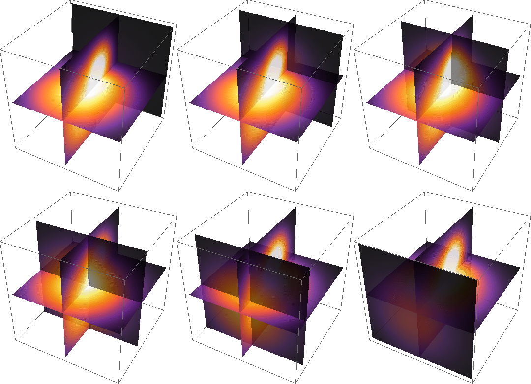
If you can afford lowering the PlotPoints, Manipulate isn't too bad, and you can make animations that look like volumetric rendering (apologies for the 300K gif):

Table[Block[{d1, d2, d3, function, options, opacity, x0, y0, z0, min, 
    max},
   {min, max} = {-9, 9};
   {x0, y0, z0} = {0., t, 0.};
   opacity = 0.9;
   function[x_, y_, z_] := 
    E^(-(x^2 + (y - 2)^2 + (z - 3)^2)/10) + 
     E^(-((x + 1)^2 + (y + 2)^2 + (z + 2)^2)/45);
   options = 
    Sequence @@ {PlotPoints -> 25, Mesh -> None, 
      ColorFunctionScaling -> False, 
      ColorFunction -> "SunsetColors"};
   d1 = First@
      DensityPlot[function[x, y, z0], {x, min, max}, {y, min, max}, 
       Evaluate@options] /. {x_?AtomQ, y_?AtomQ} -> {x, y, z0};
   d2 = First@
      DensityPlot[function[x, y0, z], {x, min, max}, {z, min, max}, 
       Evaluate@options] /. {x_?AtomQ, z_?AtomQ} -> {x, y0, z};
   d3 = First@
      DensityPlot[function[x0, y, z], {y, min, max}, {z, min, max}, 
       Evaluate@options] /. {y_?AtomQ, z_?AtomQ} -> {x0, y, z};
   Show[Graphics3D[{d1, d2, d3}, Lighting -> "Neutral"] /. 
     GraphicsComplex[xx__] -> {Opacity[opacity], 
       GraphicsComplex[xx]}]
   ], {t, 9, -9, -1.5}];
Export["3d.gif", %];