Commonmark migration
Source Link

I have some [data][1]data and want to fit it to Planck's law for black body radiation. The problem is that Mathematica does not give me the correct coefficients.

[![enter image description here][2]][2]enter image description here

I get: [![enter image description here][3]][3]enter image description here

I get out what I need.
What is it I am doing wrong? I did not really understood it in answers. Thank you. [1]: https://pastebin.com/MGEzkeC3 [2]: https://i.sstatic.net/sCkM5.png [3]: https://i.sstatic.net/QzrRD.png
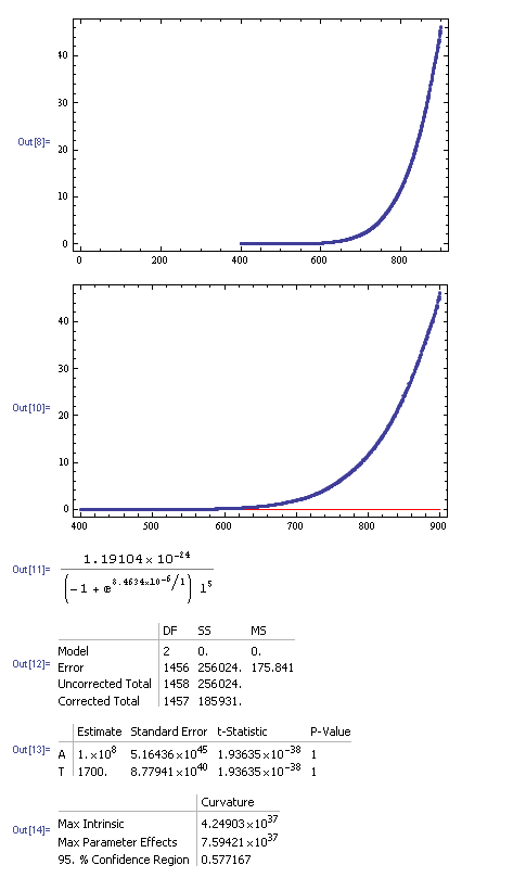
I have some [data][1] and want to fit it to Planck's law for black body radiation. The problem is that Mathematica does not give me the correct coefficients.

[![enter image description here][2]][2]

I get: [![enter image description here][3]][3]

I get out what I need.
What is it I am doing wrong? I did not really understood it in answers. Thank you. [1]: https://pastebin.com/MGEzkeC3 [2]: https://i.sstatic.net/sCkM5.png [3]: https://i.sstatic.net/QzrRD.png
I have some data and want to fit it to Planck's law for black body radiation. The problem is that Mathematica does not give me the correct coefficients.

enter image description here

I get: enter image description here

I get out what I need.
What is it I am doing wrong? I did not really understood it in answers. Thank you.

added 2026 characters in body
Source Link
Andra
  • 91
  • 7

Sorry guys for forgetting to write down constants. And my data is only the part of Black Body radiation law. And unit of x-axis is nanometers(nm), and y-axis (uW/cm^2/nm).
Update: As suggested by @JimB, I changed my fitting function. I tried to use @JimB suggested function, but for me easier was different one, because I need to find out temperature (Te). Here is the code:

h = 6.62607004*10^(-34);
c = 299792458;
kb = 1.38064852*10^(-23);
b = 2*6.62607004*10^(-34)*299792458^2*Pi;
d = (6.62607004*10^(-34)*299792458)/(1.38064852*10^(-23));
dati = ImportString[Import["H2liesma.txt"], "Table"];
Plankulis[la_, Te_, G_, b_, d_] := (1/G)*(b/(la^5*(Exp[d/(la*Te)] - 1)));
Pfit3 = FindFit[dati, 
   Plankulis[la, Te, G, b, d], {G, 1*10^(9)}, { Te, 1500} , la];
Show[Plot[Pfit3[la], {la, 400, 900}, PlotStyle -> Red, 
  PlotRange -> All], ListPlot[dati], Frame -> True]

I get:

  FindFit::nonopt: Options expected (instead of la) beyond position 4 in FindFit[{{400.035,-0.00759963},{400.409,0.0136996},{400.783,-0.000465753},{401.157,0.00636862},{401.531,0.0205706},{401.904,0.0257837},{402.278,0.0298773},{402.652,0.00226108},{403.025,0.0188769},{403.399,-0.0230916},{403.772,-0.00365794},{404.146,0.00856837},<<28>>,{414.961,-0.00272152},{415.333,-0.00222349},{415.706,-0.00943255},{416.078,-0.00921836},{416.45,0.00204648},{416.823,-0.0261218},{417.195,-0.00775242},{417.567,0.0140285},{417.939,-0.00992257},{418.311,-0.00711655},<<1408>>},<<24>>/<<1>>,{<<1>>},<<1>>,la]. An option must be a rule or a list of rules. >>

When I write analitical solution for my function:

b = 2*6.62607004*10^(-34)*299792458^2*Pi;
d = (6.62607004*10^(-34)*299792458)/(1.38064852*10^(-23));
Plankulis1[la_] := (1/G)*(b/(la^5*(Exp[d/(la*Te)] - 1)));
Te = 1500;
G = 1*10^(9);
Plankulis[G, b, la, d, Te]
Plot[Plankulis1[la], {la, 400*10^(-9), 
  700*10^(-8)}, {PlotRange -> Full},  Frame -> True]

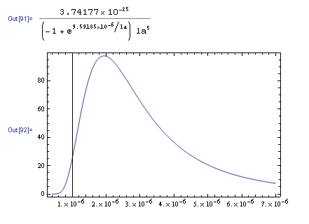
I get: [![enter image description here][3]][3]

I get out what I need.
What is it I am doing wrong? I did not really understood it in answers. Thank you. [1]: https://pastebin.com/MGEzkeC3 [2]: https://i.sstatic.net/sCkM5.png [3]: https://i.sstatic.net/QzrRD.png

Sorry guys for forgetting to write down constants. And my data is only the part of Black Body radiation law. And unit of x-axis is nanometers(nm), and y-axis (uW/cm^2/nm). [1]: https://pastebin.com/MGEzkeC3 [2]: https://i.sstatic.net/sCkM5.png

Sorry guys for forgetting to write down constants. And my data is only the part of Black Body radiation law. And unit of x-axis is nanometers(nm), and y-axis (uW/cm^2/nm).
Update: As suggested by @JimB, I changed my fitting function. I tried to use @JimB suggested function, but for me easier was different one, because I need to find out temperature (Te). Here is the code:

h = 6.62607004*10^(-34);
c = 299792458;
kb = 1.38064852*10^(-23);
b = 2*6.62607004*10^(-34)*299792458^2*Pi;
d = (6.62607004*10^(-34)*299792458)/(1.38064852*10^(-23));
dati = ImportString[Import["H2liesma.txt"], "Table"];
Plankulis[la_, Te_, G_, b_, d_] := (1/G)*(b/(la^5*(Exp[d/(la*Te)] - 1)));
Pfit3 = FindFit[dati, 
   Plankulis[la, Te, G, b, d], {G, 1*10^(9)}, { Te, 1500} , la];
Show[Plot[Pfit3[la], {la, 400, 900}, PlotStyle -> Red, 
  PlotRange -> All], ListPlot[dati], Frame -> True]

I get:

  FindFit::nonopt: Options expected (instead of la) beyond position 4 in FindFit[{{400.035,-0.00759963},{400.409,0.0136996},{400.783,-0.000465753},{401.157,0.00636862},{401.531,0.0205706},{401.904,0.0257837},{402.278,0.0298773},{402.652,0.00226108},{403.025,0.0188769},{403.399,-0.0230916},{403.772,-0.00365794},{404.146,0.00856837},<<28>>,{414.961,-0.00272152},{415.333,-0.00222349},{415.706,-0.00943255},{416.078,-0.00921836},{416.45,0.00204648},{416.823,-0.0261218},{417.195,-0.00775242},{417.567,0.0140285},{417.939,-0.00992257},{418.311,-0.00711655},<<1408>>},<<24>>/<<1>>,{<<1>>},<<1>>,la]. An option must be a rule or a list of rules. >>

When I write analitical solution for my function:

b = 2*6.62607004*10^(-34)*299792458^2*Pi;
d = (6.62607004*10^(-34)*299792458)/(1.38064852*10^(-23));
Plankulis1[la_] := (1/G)*(b/(la^5*(Exp[d/(la*Te)] - 1)));
Te = 1500;
G = 1*10^(9);
Plankulis[G, b, la, d, Te]
Plot[Plankulis1[la], {la, 400*10^(-9), 
  700*10^(-8)}, {PlotRange -> Full},  Frame -> True]

I get: [![enter image description here][3]][3]

I get out what I need.
What is it I am doing wrong? I did not really understood it in answers. Thank you. [1]: https://pastebin.com/MGEzkeC3 [2]: https://i.sstatic.net/sCkM5.png [3]: https://i.sstatic.net/QzrRD.png

added 147 characters in body
Source Link
Andra
  • 91
  • 7

I have some data[data][1] and want to fit it to Planck's law for black body radiation. The problem is that Mathematica does not give me the correct coefficients.

When I evaluate

dati = Import["https://pastebin.com/raw/MGEzkeC3", "Table"];
(*Show[ListPlot[dati,h Frame= 6.62607004*10^(->34);
c True]]*= 299792458;
kb = 1.38064852*10^(-23);
Planks[l_, T_, A_] := (1/A)*(((2*h*c^2)/l^5)*(1/(Exp[((h*c)/(l*kb*T))] - 1)));
fittesana2 = FindFit[dati, Planks[l, T, A], {T, A } , l];
Show[
  Plot[fittesana2[l], {l, 400, 900}, PlotStyle -> Red, PlotRange -> All], 
  ListPlot[dati], Frame -> True]
Pfit = NonlinearModelFit[dati, Planks[l, T, A], {{A, 1*10^8}, {T, 1700}}, l];
Show[
  Plot[Pfit[l], {l, 400, 900}, PlotStyle -> Red, PlotRange -> All],
  ListPlot[dati], Frame -> True]
Normal[Pfit]
Pfit["ANOVATable"]
Pfit["ParameterTable"]
Pfit["FitCurvatureTable"]

I get

[![enter image description here][2]][2]

Sorry guys for forgetting to write down constants. And my data is only the part of Black Body radiation law. And unit of x-axis is nanometers(nm), and y-axis (uW/cm^2/nm). [1]: https://pastebin.com/MGEzkeC3 [2]: enter image description herehttps://i.sstatic.net/sCkM5.png

I have some data and want to fit it to Planck's law for black body radiation. The problem is that Mathematica does not give me the correct coefficients.

When I evaluate

dati = Import["https://pastebin.com/raw/MGEzkeC3", "Table"];
(*Show[ListPlot[dati, Frame -> True]]*)
Planks[l_, T_, A_] := (1/A)*(((2*h*c^2)/l^5)*(1/(Exp[((h*c)/(l*kb*T))] - 1)));
fittesana2 = FindFit[dati, Planks[l, T, A], {T, A } , l];
Show[
  Plot[fittesana2[l], {l, 400, 900}, PlotStyle -> Red, PlotRange -> All], 
  ListPlot[dati], Frame -> True]
Pfit = NonlinearModelFit[dati, Planks[l, T, A], {{A, 1*10^8}, {T, 1700}}, l];
Show[
  Plot[Pfit[l], {l, 400, 900}, PlotStyle -> Red, PlotRange -> All],
  ListPlot[dati], Frame -> True]
Normal[Pfit]
Pfit["ANOVATable"]
Pfit["ParameterTable"]
Pfit["FitCurvatureTable"]

I get

enter image description here

I have some [data][1] and want to fit it to Planck's law for black body radiation. The problem is that Mathematica does not give me the correct coefficients.

When I evaluate

dati = Import["https://pastebin.com/raw/MGEzkeC3", "Table"];
h = 6.62607004*10^(-34);
c = 299792458;
kb = 1.38064852*10^(-23);
Planks[l_, T_, A_] := (1/A)*(((2*h*c^2)/l^5)*(1/(Exp[((h*c)/(l*kb*T))] - 1)));
fittesana2 = FindFit[dati, Planks[l, T, A], {T, A } , l];
Show[
  Plot[fittesana2[l], {l, 400, 900}, PlotStyle -> Red, PlotRange -> All], 
  ListPlot[dati], Frame -> True]
Pfit = NonlinearModelFit[dati, Planks[l, T, A], {{A, 1*10^8}, {T, 1700}}, l];
Show[
  Plot[Pfit[l], {l, 400, 900}, PlotStyle -> Red, PlotRange -> All],
  ListPlot[dati], Frame -> True]
Normal[Pfit]
Pfit["ANOVATable"]
Pfit["ParameterTable"]
Pfit["FitCurvatureTable"]

I get

[![enter image description here][2]][2]

Sorry guys for forgetting to write down constants. And my data is only the part of Black Body radiation law. And unit of x-axis is nanometers(nm), and y-axis (uW/cm^2/nm). [1]: https://pastebin.com/MGEzkeC3 [2]: https://i.sstatic.net/sCkM5.png

edited tags
Link
Loading
Routine clean-up
Source Link
m_goldberg
  • 108.1k
  • 16
  • 104
  • 259
Loading
edited tags
Source Link
Loading
Source Link
Andra
  • 91
  • 7
Loading