Image derivatives are susceptible to noise. To counteract this effect, you can regularize the image or data by a Gaussian kernel of standard deviation
σ. The default value isσ=0σ = 0.
In
RidgeFilter[image, σ],σis the scale of the ridges that is used to compute the derivatives in the Hessian. By default,σ=1σ = 1is used.
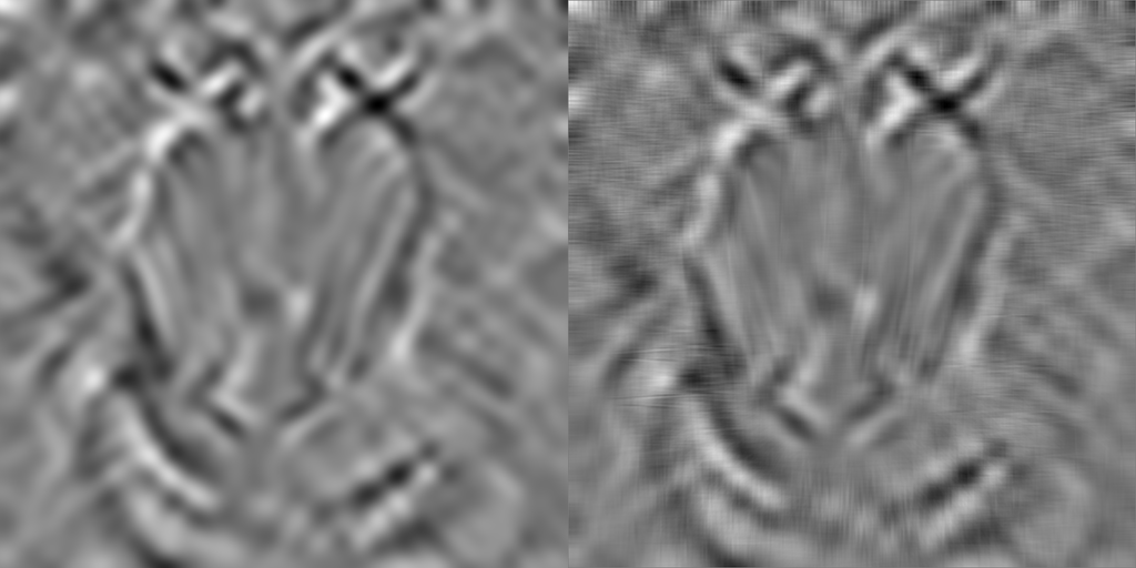
Nevertheless, combining the information from the two pages of the docs, I still can't tell what exactly the functions are doing. It sounds to me like they simply run a GaussianFilter over the image first. I can obtain results at the same scale by using 2σ2 σ as the radius of the Gaussian filter, but then I still get a lot of small scale artefacts that are missing when I use DerivativeFilter or RidgeFilter directly:
img = ColorConvert[ExampleData[{"TestImage", "Mandrill"}], "Grayscale"]
σ = 10;
ImageAssemble @ {
  ImageAdjust@DerivativeFilter[imgImageAdjust @ DerivativeFilter[img, {1, 1}, σ],
  ImageAdjust@DerivativeFilter[GaussianFilter[imgImageAdjust @ DerivativeFilter[GaussianFilter[img, 2σ]2 σ], {1, 1}]
}
GaussianFilter[image, r]uses r = σ/2r = σ/2.
All of this seems highly confusinconfusing, and there must be more to it than simply smoothing the input up front.

