added 3D phase portrait
Source Link
Chris K
  • 20.4k
  • 3
  • 39
  • 75

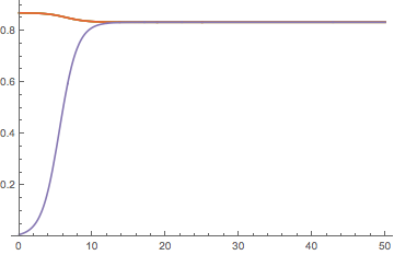
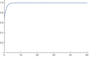
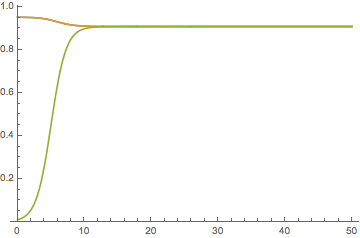
This looks like a Lotka-Volterra competition model with weak, symmetric interspecific competition. If I understand correctly, you want to build up a community by introducing new species every T=50 time steps, where the new species has initial density of 0.01 times one of the existing species.

Call me old-fashioned, but I think this is easiest to understand when handled in an iterative Do loop:

nmax = 5; (* max number of species *)
T = 50; (* period *)
nu = 0.05; (* interspecific competition coefficient *)

(* set up unknown vars and differential equations, for n species *)

vars := Table[Subscript[x, j], {j, n}];
eqns := Table[Subscript[x, j]'[t] == Subscript[x, j][t]
  (1 - Subscript[x, j][t]- nu (Sum[Subscript[x, k][t] Boole[k != j], {k, n}]))
, {j, n}];

(* initial ICs *)
ics = {Subscript[x, 1][0] == 0.7};

(* main loop *)
Do[
  (* solve for n species *)
  sol[n] = NDSolve[{eqns, ics}, vars, {t, 0, T}][[1]];
  (* plot dynamics *)
  Print[Plot[Evaluate[Table[Subscript[x, j][t], {j, n}] /. sol[n]], {t, 0, T}, PlotRange -> {0, All}]];

  (* set up ICs for n=n+1 species *)
  ics = Join[
    Table[Subscript[x, j][0] == Evaluate[Subscript[x, j][T] /. sol[n]], {j, n}],
    {Subscript[x, n + 1][0] == Evaluate[0.01 Subscript[x, RandomInteger[{1, n}]][T] /. sol[n]]}
   ];
, {n, nmax}]
Mathematica graphics Mathematica graphics Mathematica graphics Mathematica graphics Mathematica graphics

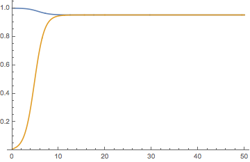
Not sure how interesting this is, since I believe this symmetric LV system has a globally stable equilibrium at $x_i=1/(1-(n-1)nu)$ as long as $0<nu<1$, but you could use this as a basis for more interesting explorations of community assembly.

Edit

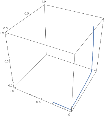
Here's a 3D phase portrait of the first three periods for @MMM:

Show[
  ParametricPlot3D[Evaluate[{Subscript[x, 1][t], 0, 0} /. sol[1]], {t, 0, T}],
  ParametricPlot3D[Evaluate[{Subscript[x, 1][t], Subscript[x, 2][t], 0} /. sol[2]], {t, 0, T}],
  ParametricPlot3D[Evaluate[{Subscript[x, 1][t], Subscript[x, 2][t], Subscript[x, 3][t]} /. sol[3]], {t, 0, T}],
  PlotRange -> {{0, 1}, {0, 1}, {0, 1}}
]

Mathematica graphics

This looks like a Lotka-Volterra competition model with weak, symmetric interspecific competition. If I understand correctly, you want to build up a community by introducing new species every T=50 time steps, where the new species has initial density of 0.01 times one of the existing species.

Call me old-fashioned, but I think this is easiest to understand when handled in an iterative Do loop:

nmax = 5; (* max number of species *)
T = 50; (* period *)
nu = 0.05; (* interspecific competition coefficient *)

(* set up unknown vars and differential equations, for n species *)

vars := Table[Subscript[x, j], {j, n}];
eqns := Table[Subscript[x, j]'[t] == Subscript[x, j][t]
  (1 - Subscript[x, j][t]- nu (Sum[Subscript[x, k][t] Boole[k != j], {k, n}]))
, {j, n}];

(* initial ICs *)
ics = {Subscript[x, 1][0] == 0.7};

(* main loop *)
Do[
  (* solve for n species *)
  sol[n] = NDSolve[{eqns, ics}, vars, {t, 0, T}][[1]];
  (* plot dynamics *)
  Print[Plot[Evaluate[Table[Subscript[x, j][t], {j, n}] /. sol[n]], {t, 0, T}, PlotRange -> {0, All}]];

  (* set up ICs for n=n+1 species *)
  ics = Join[
    Table[Subscript[x, j][0] == Evaluate[Subscript[x, j][T] /. sol[n]], {j, n}],
    {Subscript[x, n + 1][0] == Evaluate[0.01 Subscript[x, RandomInteger[{1, n}]][T] /. sol[n]]}
   ];
, {n, nmax}]
Mathematica graphics Mathematica graphics Mathematica graphics Mathematica graphics Mathematica graphics

Not sure how interesting this is, since I believe this symmetric LV system has a globally stable equilibrium at $x_i=1/(1-(n-1)nu)$ as long as $0<nu<1$, but you could use this as a basis for more interesting explorations of community assembly.

This looks like a Lotka-Volterra competition model with weak, symmetric interspecific competition. If I understand correctly, you want to build up a community by introducing new species every T=50 time steps, where the new species has initial density of 0.01 times one of the existing species.

Call me old-fashioned, but I think this is easiest to understand when handled in an iterative Do loop:

nmax = 5; (* max number of species *)
T = 50; (* period *)
nu = 0.05; (* interspecific competition coefficient *)

(* set up unknown vars and differential equations, for n species *)

vars := Table[Subscript[x, j], {j, n}];
eqns := Table[Subscript[x, j]'[t] == Subscript[x, j][t]
  (1 - Subscript[x, j][t]- nu (Sum[Subscript[x, k][t] Boole[k != j], {k, n}]))
, {j, n}];

(* initial ICs *)
ics = {Subscript[x, 1][0] == 0.7};

(* main loop *)
Do[
  (* solve for n species *)
  sol[n] = NDSolve[{eqns, ics}, vars, {t, 0, T}][[1]];
  (* plot dynamics *)
  Print[Plot[Evaluate[Table[Subscript[x, j][t], {j, n}] /. sol[n]], {t, 0, T}, PlotRange -> {0, All}]];

  (* set up ICs for n=n+1 species *)
  ics = Join[
    Table[Subscript[x, j][0] == Evaluate[Subscript[x, j][T] /. sol[n]], {j, n}],
    {Subscript[x, n + 1][0] == Evaluate[0.01 Subscript[x, RandomInteger[{1, n}]][T] /. sol[n]]}
   ];
, {n, nmax}]
Mathematica graphics Mathematica graphics Mathematica graphics Mathematica graphics Mathematica graphics

Not sure how interesting this is, since I believe this symmetric LV system has a globally stable equilibrium at $x_i=1/(1-(n-1)nu)$ as long as $0<nu<1$, but you could use this as a basis for more interesting explorations of community assembly.

Edit

Here's a 3D phase portrait of the first three periods for @MMM:

Show[
  ParametricPlot3D[Evaluate[{Subscript[x, 1][t], 0, 0} /. sol[1]], {t, 0, T}],
  ParametricPlot3D[Evaluate[{Subscript[x, 1][t], Subscript[x, 2][t], 0} /. sol[2]], {t, 0, T}],
  ParametricPlot3D[Evaluate[{Subscript[x, 1][t], Subscript[x, 2][t], Subscript[x, 3][t]} /. sol[3]], {t, 0, T}],
  PlotRange -> {{0, 1}, {0, 1}, {0, 1}}
]

Mathematica graphics

Source Link
Chris K
  • 20.4k
  • 3
  • 39
  • 75

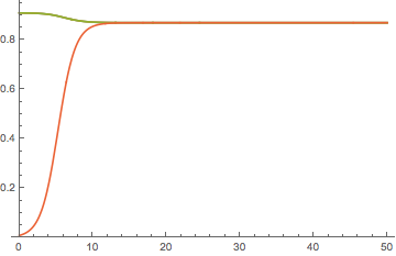
This looks like a Lotka-Volterra competition model with weak, symmetric interspecific competition. If I understand correctly, you want to build up a community by introducing new species every T=50 time steps, where the new species has initial density of 0.01 times one of the existing species.

Call me old-fashioned, but I think this is easiest to understand when handled in an iterative Do loop:

nmax = 5; (* max number of species *)
T = 50; (* period *)
nu = 0.05; (* interspecific competition coefficient *)

(* set up unknown vars and differential equations, for n species *)

vars := Table[Subscript[x, j], {j, n}];
eqns := Table[Subscript[x, j]'[t] == Subscript[x, j][t]
  (1 - Subscript[x, j][t]- nu (Sum[Subscript[x, k][t] Boole[k != j], {k, n}]))
, {j, n}];

(* initial ICs *)
ics = {Subscript[x, 1][0] == 0.7};

(* main loop *)
Do[
  (* solve for n species *)
  sol[n] = NDSolve[{eqns, ics}, vars, {t, 0, T}][[1]];
  (* plot dynamics *)
  Print[Plot[Evaluate[Table[Subscript[x, j][t], {j, n}] /. sol[n]], {t, 0, T}, PlotRange -> {0, All}]];

  (* set up ICs for n=n+1 species *)
  ics = Join[
    Table[Subscript[x, j][0] == Evaluate[Subscript[x, j][T] /. sol[n]], {j, n}],
    {Subscript[x, n + 1][0] == Evaluate[0.01 Subscript[x, RandomInteger[{1, n}]][T] /. sol[n]]}
   ];
, {n, nmax}]
Mathematica graphics Mathematica graphics Mathematica graphics Mathematica graphics Mathematica graphics

Not sure how interesting this is, since I believe this symmetric LV system has a globally stable equilibrium at $x_i=1/(1-(n-1)nu)$ as long as $0<nu<1$, but you could use this as a basis for more interesting explorations of community assembly.