deleted 1 character in body
Source Link
L.K.
  • 693
  • 1
  • 7
  • 17

I have a matrix whose eigenvalues have to be plotted. I am using two techniques but they are not the same. Please guide me on this.

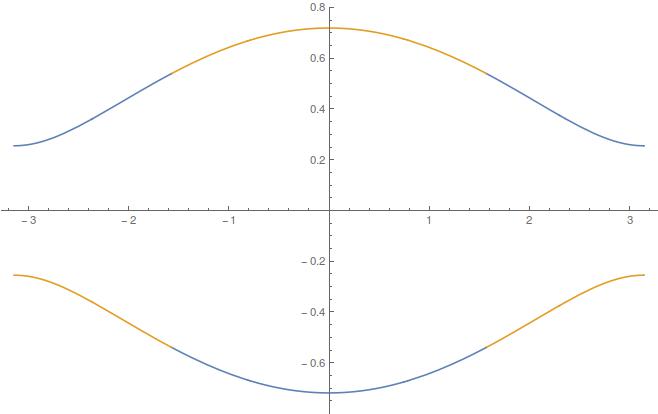
Here is first command or code used for plotting the eigenvalues(two in my case)

a := 1;
SM[j1_, j2_, k_] := {{0, -(j1 + j2*Exp[I*k*a])}, {-(j1 + (j2*Exp[-I*k*a])), 
    0}};
eigenen[j1_, j2_, k_] := Module[{EV1}, EV1 = Eigenvalues[SM[j1, j2, k]];
  Plot[EV1, {k, -\[Pi]/a, \[Pi]/a}, PlotLegends -> "Expressions"]]
Manipulate[eigenen[j1, j2, k], {j1, 0.1, 1}, {j2, 0.1, 1}]

Result is (j1>j2, you can take j1=0.3, j2=0.1) enter image description here
Second used code

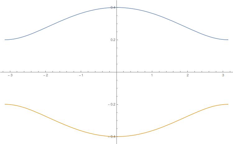
a:=1;
PowerExpand[FullSimplify[Eigenvalues[ {{0, -(j1 + j2*Exp[I*ka])},{-(j1 + j2*Exp[-I*ka]), 0}} ]]]

Out:= {-Sqrt[j1^2 + j2^2 + 2 j1 j2 Cos[ka]], Sqrt[j1^2 + j2^2 + 2 j1 j2 Cos[ka]]}
Manipulate[Plot[{Sqrt[(j1^2 + j2^2 + 2 j1 j2 Cos[k*a])], -Sqrt[(j1^2 + j2^2 + 2 j1 j2 Cos[k*a])]}, {k, -\[Pi]/a, \[Pi]/a}, 
  PlotLegends -> "Expressions"], {j1, 0.1, 1}, {j2, 0.1, 1}]

For this result is (j1>j2, you can take j1=0.3, j2=0.1) enter image description here
I have no idea about the difference but I will be using first code more often as I later have to deal with large matrices(40$\times$ 40), where I can't simply write the eigenvalues. Is there any effective or similar code where this problem can be resolved?

My queries(to summarise):
(i) Reason(s) for the difference in the plots.
(ii) Anyway the secondfirst code can be resolved to give similar results as Ist one(those are expected ones), not as the IIndIst ones.

I have a matrix whose eigenvalues have to be plotted. I am using two techniques but they are not the same. Please guide me on this.

Here is first command or code used for plotting the eigenvalues(two in my case)

a := 1;
SM[j1_, j2_, k_] := {{0, -(j1 + j2*Exp[I*k*a])}, {-(j1 + (j2*Exp[-I*k*a])), 
    0}};
eigenen[j1_, j2_, k_] := Module[{EV1}, EV1 = Eigenvalues[SM[j1, j2, k]];
  Plot[EV1, {k, -\[Pi]/a, \[Pi]/a}, PlotLegends -> "Expressions"]]
Manipulate[eigenen[j1, j2, k], {j1, 0.1, 1}, {j2, 0.1, 1}]

Result is (j1>j2, you can take j1=0.3, j2=0.1) enter image description here

Second used code

a:=1;
PowerExpand[FullSimplify[Eigenvalues[ {{0, -(j1 + j2*Exp[I*ka])},{-(j1 + j2*Exp[-I*ka]), 0}} ]]]

Out:= {-Sqrt[j1^2 + j2^2 + 2 j1 j2 Cos[ka]], Sqrt[j1^2 + j2^2 + 2 j1 j2 Cos[ka]]}
Manipulate[Plot[{Sqrt[(j1^2 + j2^2 + 2 j1 j2 Cos[k*a])], -Sqrt[(j1^2 + j2^2 + 2 j1 j2 Cos[k*a])]}, {k, -\[Pi]/a, \[Pi]/a}, 
  PlotLegends -> "Expressions"], {j1, 0.1, 1}, {j2, 0.1, 1}]

For this result is (j1>j2, you can take j1=0.3, j2=0.1) enter image description here

I have no idea about the difference but I will be using first code more often as I later have to deal with large matrices(40$\times$ 40), where I can't simply write the eigenvalues. Is there any effective or similar code where this problem can be resolved?

My queries(to summarise):
(i) Reason(s) for the difference in the plots.
(ii) Anyway the second code can be resolved to give similar results as Ist one(those are expected ones), not the IInd ones.

I have a matrix whose eigenvalues have to be plotted. I am using two techniques but they are not the same. Please guide me on this.

Here is first command or code used for plotting the eigenvalues(two in my case)

a := 1;
SM[j1_, j2_, k_] := {{0, -(j1 + j2*Exp[I*k*a])}, {-(j1 + (j2*Exp[-I*k*a])), 
    0}};
eigenen[j1_, j2_, k_] := Module[{EV1}, EV1 = Eigenvalues[SM[j1, j2, k]];
  Plot[EV1, {k, -\[Pi]/a, \[Pi]/a}, PlotLegends -> "Expressions"]]
Manipulate[eigenen[j1, j2, k], {j1, 0.1, 1}, {j2, 0.1, 1}]

Result is (j1>j2, you can take j1=0.3, j2=0.1) enter image description here

Second used code

a:=1;
PowerExpand[FullSimplify[Eigenvalues[ {{0, -(j1 + j2*Exp[I*ka])},{-(j1 + j2*Exp[-I*ka]), 0}} ]]]

Out:= {-Sqrt[j1^2 + j2^2 + 2 j1 j2 Cos[ka]], Sqrt[j1^2 + j2^2 + 2 j1 j2 Cos[ka]]}
Manipulate[Plot[{Sqrt[(j1^2 + j2^2 + 2 j1 j2 Cos[k*a])], -Sqrt[(j1^2 + j2^2 + 2 j1 j2 Cos[k*a])]}, {k, -\[Pi]/a, \[Pi]/a}, 
  PlotLegends -> "Expressions"], {j1, 0.1, 1}, {j2, 0.1, 1}]

For this result is (j1>j2, you can take j1=0.3, j2=0.1) enter image description here

I have no idea about the difference but I will be using first code more often as I later have to deal with large matrices(40$\times$ 40), where I can't simply write the eigenvalues. Is there any effective or similar code where this problem can be resolved?

My queries(to summarise):
(i) Reason(s) for the difference in the plots.
(ii) Anyway the first code can be resolved to give similar results as Ist one(those are expected ones), not as the Ist ones.

edited tags
Link
deleted 3 characters in body
Source Link
L.K.
  • 693
  • 1
  • 7
  • 17

I have a matrix whose eigenvalues have to be plotted. I am using two techniques but they are not the same. Please guide me on this.

Here is first command or code used for plotting the eigenvalues(two in my case)

a := 1;
SM[j1_, j2_, k_] := {{0, -(j1 + j2*Exp[I*k*a])}, {-(j1 + (j2*Exp[-I*k*a])), 
    0}};
eigenen[j1_, j2_, k_] := Module[{EV1}, EV1 = Eigenvalues[SM[j1, j2, k]];
  Plot[EV1, {k, -\[Pi]/a, \[Pi]/a}, PlotLegends -> "Expressions"]]
Manipulate[eigenen[j1, j2, k], {j1, 0.1, 1}, {j2, 0.1, 1}]

Result is (j1>j2, you can take j1=0.3, j2=0.1) enter image description here

Second used code

a:=1;
PowerExpand[FullSimplify[Eigenvalues[ {{0, -(j1 + j2*Exp[I*ka])},{-(j1 + j2*Exp[-I*ka]), 0}} ]]]

Out:= {-Sqrt[j1^2 + j2^2 + 2 j1 j2 Cos[ka]], Sqrt[j1^2 + j2^2 + 2 j1 j2 Cos[ka]]}
Manipulate[Plot[{Sqrt[(j1^2 + j2^2 + 2 j1 j2 Cos[k*a])], -Sqrt[(j1^2 + j2^2 + 2 j1 j2 Cos[k*a])]}, {k, -\[Pi]/a, \[Pi]/a}, 
  PlotLegends -> "Expressions"], {j1, 0.1, 1}, {j2, 0.1, 1}]

For this result is (j1>j2, you can take j1=0.3, j2=0.1) enter image description here

I have no idea about the difference but I will be using first code more often as I later have to deal with large matrices(40$\times$ 40), where I can't simply write the eigenvalues. OrIs there is any effective or similar code where this problem can be resolved.?

My queries(to summarise):
(i) Reason(s) for the difference in the plots.
(ii) Anyway the second code can be resolved to give similar results as Ist one(those are expected ones), not the IInd ones.

I have a matrix whose eigenvalues have to be plotted. I am using two techniques but they are not the same. Please guide me on this.

Here is first command or code used for plotting the eigenvalues(two in my case)

a := 1;
SM[j1_, j2_, k_] := {{0, -(j1 + j2*Exp[I*k*a])}, {-(j1 + (j2*Exp[-I*k*a])), 
    0}};
eigenen[j1_, j2_, k_] := Module[{EV1}, EV1 = Eigenvalues[SM[j1, j2, k]];
  Plot[EV1, {k, -\[Pi]/a, \[Pi]/a}, PlotLegends -> "Expressions"]]
Manipulate[eigenen[j1, j2, k], {j1, 0.1, 1}, {j2, 0.1, 1}]

Result is (j1>j2, you can take j1=0.3, j2=0.1) enter image description here

Second used code

a:=1;
PowerExpand[FullSimplify[Eigenvalues[ {{0, -(j1 + j2*Exp[I*ka])},{-(j1 + j2*Exp[-I*ka]), 0}} ]]]

Out:= {-Sqrt[j1^2 + j2^2 + 2 j1 j2 Cos[ka]], Sqrt[j1^2 + j2^2 + 2 j1 j2 Cos[ka]]}
Manipulate[Plot[{Sqrt[(j1^2 + j2^2 + 2 j1 j2 Cos[k*a])], -Sqrt[(j1^2 + j2^2 + 2 j1 j2 Cos[k*a])]}, {k, -\[Pi]/a, \[Pi]/a}, 
  PlotLegends -> "Expressions"], {j1, 0.1, 1}, {j2, 0.1, 1}]

For this result is (j1>j2, you can take j1=0.3, j2=0.1) enter image description here

I have no idea about the difference but I will be using first code more often as I later have to deal with large matrices(40$\times$ 40), where I can't simply write the eigenvalues. Or there is any effective or similar code where this problem can be resolved.

My queries(to summarise):
(i) Reason(s) for the difference in the plots.
(ii) Anyway the second code can be resolved to give similar results as Ist one(those are expected ones), not the IInd ones.

I have a matrix whose eigenvalues have to be plotted. I am using two techniques but they are not the same. Please guide me on this.

Here is first command or code used for plotting the eigenvalues(two in my case)

a := 1;
SM[j1_, j2_, k_] := {{0, -(j1 + j2*Exp[I*k*a])}, {-(j1 + (j2*Exp[-I*k*a])), 
    0}};
eigenen[j1_, j2_, k_] := Module[{EV1}, EV1 = Eigenvalues[SM[j1, j2, k]];
  Plot[EV1, {k, -\[Pi]/a, \[Pi]/a}, PlotLegends -> "Expressions"]]
Manipulate[eigenen[j1, j2, k], {j1, 0.1, 1}, {j2, 0.1, 1}]

Result is (j1>j2, you can take j1=0.3, j2=0.1) enter image description here

Second used code

a:=1;
PowerExpand[FullSimplify[Eigenvalues[ {{0, -(j1 + j2*Exp[I*ka])},{-(j1 + j2*Exp[-I*ka]), 0}} ]]]

Out:= {-Sqrt[j1^2 + j2^2 + 2 j1 j2 Cos[ka]], Sqrt[j1^2 + j2^2 + 2 j1 j2 Cos[ka]]}
Manipulate[Plot[{Sqrt[(j1^2 + j2^2 + 2 j1 j2 Cos[k*a])], -Sqrt[(j1^2 + j2^2 + 2 j1 j2 Cos[k*a])]}, {k, -\[Pi]/a, \[Pi]/a}, 
  PlotLegends -> "Expressions"], {j1, 0.1, 1}, {j2, 0.1, 1}]

For this result is (j1>j2, you can take j1=0.3, j2=0.1) enter image description here

I have no idea about the difference but I will be using first code more often as I later have to deal with large matrices(40$\times$ 40), where I can't simply write the eigenvalues. Is there any effective or similar code where this problem can be resolved?

My queries(to summarise):
(i) Reason(s) for the difference in the plots.
(ii) Anyway the second code can be resolved to give similar results as Ist one(those are expected ones), not the IInd ones.

Source Link
L.K.
  • 693
  • 1
  • 7
  • 17
Loading