Revisions to Predicting the initial conditions of orbits inside a closed curve

replaced http://mathematica.stackexchange.com/ with https://mathematica.stackexchange.com/

Source Link

edited Apr 13, 2017 at 12:56

1

I have a data file containing the four orbital element $(x,y,p_x,p_y)$ of a two-dimensional closed loop orbit. Note that the exact implicit equation of the orbit is not known.

The plot of the 2D orbit on the $(x,y)$ plane

data = Import["lyap_4d.dat", "Table"];
d00 = data[[All, {1, 2}]];
 
C0 = ListLinePlot[d00, AspectRatio -> 1, PlotRange -> All, 
     Frame -> True, Axes -> False, PlotStyle -> {Black, Thick}]

Now let's define a rectangular grid of initial conditions around this orbit

data = Flatten[Table[{i, j}, {i, 0.785, 1.135, 0.005}, 
       {j, -0.45, 0.45, 0.005}], 1];
nic = Length[data]
L0 = ListPlot[data, PlotStyle -> {Blue, PointSize[0.001]}];
plot1 = Show[{L0, C0}]

Finally, we determine which of the initial conditions are inside the orbit using the code provided here here

poly = Cases[Normal@C0, Line[x_] :> x, Infinity];
inPolyQ[poly_, pt_] := Graphics`Mesh`PointWindingNumber[poly, pt] =!= 0
data2 = Select[data, inPolyQ[poly[[1]], #] &];
nic2 = Length[data2]
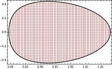
L1 = ListPlot[data2, PlotStyle -> {Red, PointSize[0.001]}];
plot2 = Show[{L1, C0}, Frame -> True, Axes -> False]

The list data2 contains all the $(x_0,y_0)$ initial conditions inside the orbit.

My question is the following: For the boundary orbit the $p_x$ and $p_y$ values are known. How can I use these values so as to predict in a way the $(p_{x0},p_{y0})$ of the orbits with initial conditions inside the orbit? In other words, how can I interpolate the $p_x$ and $p_y$ of the orbit by taking into account the values of the boundary?

I use version 9.0 of Mathematica in Win XP SP3.

Many thanks in advance!

I have a data file containing the four orbital element $(x,y,p_x,p_y)$ of a two-dimensional closed loop orbit. Note that the exact implicit equation of the orbit is not known.

The plot of the 2D orbit on the $(x,y)$ plane

data = Import["lyap_4d.dat", "Table"];
d00 = data[[All, {1, 2}]];
 
C0 = ListLinePlot[d00, AspectRatio -> 1, PlotRange -> All, 
     Frame -> True, Axes -> False, PlotStyle -> {Black, Thick}]

Now let's define a rectangular grid of initial conditions around this orbit

data = Flatten[Table[{i, j}, {i, 0.785, 1.135, 0.005}, 
       {j, -0.45, 0.45, 0.005}], 1];
nic = Length[data]
L0 = ListPlot[data, PlotStyle -> {Blue, PointSize[0.001]}];
plot1 = Show[{L0, C0}]

Finally, we determine which of the initial conditions are inside the orbit using the code provided here

poly = Cases[Normal@C0, Line[x_] :> x, Infinity];
inPolyQ[poly_, pt_] := Graphics`Mesh`PointWindingNumber[poly, pt] =!= 0
data2 = Select[data, inPolyQ[poly[[1]], #] &];
nic2 = Length[data2]
L1 = ListPlot[data2, PlotStyle -> {Red, PointSize[0.001]}];
plot2 = Show[{L1, C0}, Frame -> True, Axes -> False]

The list data2 contains all the $(x_0,y_0)$ initial conditions inside the orbit.

My question is the following: For the boundary orbit the $p_x$ and $p_y$ values are known. How can I use these values so as to predict in a way the $(p_{x0},p_{y0})$ of the orbits with initial conditions inside the orbit? In other words, how can I interpolate the $p_x$ and $p_y$ of the orbit by taking into account the values of the boundary?

I use version 9.0 of Mathematica in Win XP SP3.

Many thanks in advance!

I have a data file containing the four orbital element $(x,y,p_x,p_y)$ of a two-dimensional closed loop orbit. Note that the exact implicit equation of the orbit is not known.

The plot of the 2D orbit on the $(x,y)$ plane

data = Import["lyap_4d.dat", "Table"];
d00 = data[[All, {1, 2}]];
 
C0 = ListLinePlot[d00, AspectRatio -> 1, PlotRange -> All, 
     Frame -> True, Axes -> False, PlotStyle -> {Black, Thick}]

Now let's define a rectangular grid of initial conditions around this orbit

data = Flatten[Table[{i, j}, {i, 0.785, 1.135, 0.005}, 
       {j, -0.45, 0.45, 0.005}], 1];
nic = Length[data]
L0 = ListPlot[data, PlotStyle -> {Blue, PointSize[0.001]}];
plot1 = Show[{L0, C0}]

Finally, we determine which of the initial conditions are inside the orbit using the code provided here

poly = Cases[Normal@C0, Line[x_] :> x, Infinity];
inPolyQ[poly_, pt_] := Graphics`Mesh`PointWindingNumber[poly, pt] =!= 0
data2 = Select[data, inPolyQ[poly[[1]], #] &];
nic2 = Length[data2]
L1 = ListPlot[data2, PlotStyle -> {Red, PointSize[0.001]}];
plot2 = Show[{L1, C0}, Frame -> True, Axes -> False]

The list data2 contains all the $(x_0,y_0)$ initial conditions inside the orbit.

My question is the following: For the boundary orbit the $p_x$ and $p_y$ values are known. How can I use these values so as to predict in a way the $(p_{x0},p_{y0})$ of the orbits with initial conditions inside the orbit? In other words, how can I interpolate the $p_x$ and $p_y$ of the orbit by taking into account the values of the boundary?

I use version 9.0 of Mathematica in Win XP SP3.

Many thanks in advance!

added 137 characters in body

Source Link

edited Jun 23, 2016 at 13:54

Vaggelis_Z

8.8k
6
35
81

I have a data file containing the four orbital element $(x,y,p_x,p_y)$ of a two-dimensional closed loop orbit. Note that the exact implicit equation of the orbit is not known.

The plot of the 2D orbit on the $(x,y)$ plane

data = Import["lyap_4d.dat", "Table"];
d00 = data[[All, {1, 2}]];
 
C0 = ListLinePlot[d00, AspectRatio -> 1, PlotRange -> All, 
     Frame -> True, Axes -> False, PlotStyle -> {Black, Thick}]

Now let's define a rectangular grid of initial conditions around this orbit

data = Flatten[Table[{i, j}, {i, 0.785, 1.135, 0.005}, 
       {j, -0.45, 0.45, 0.005}], 1];
nic = Length[data]
L0 = ListPlot[data, PlotStyle -> {Blue, PointSize[0.001]}];
plot1 = Show[{L0, C0}]

Finally, we determine which of the initial conditions are inside the orbit using the code provided here

poly = Cases[Normal@C0, Line[x_] :> x, Infinity];
inPolyQ[poly_, pt_] := Graphics`Mesh`PointWindingNumber[poly, pt] =!= 0
data2 = Select[data, inPolyQ[poly[[1]], #] &];
nic2 = Length[data2]
L1 = ListPlot[data2, PlotStyle -> {Red, PointSize[0.001]}];
plot2 = Show[{L1, C0}, Frame -> True, Axes -> False]

The list data2 contains all the $(x_0,y_0)$ initial conditions inside the orbit.

My question is the following: For the boundary orbit the $p_x$ and $p_y$ values are known. How can I use these values so as to predict in a way the $(p_{x0},p_{y0})$ of the orbits with initial conditions inside the orbit? In other words, how can I interpolate the $p_x$ and $p_y$ of the orbit by taking into account the values of the boundary?

I use version 9.0 of Mathematica in Win XP SP3.

Many thanks in advance!

I have a data file containing the four orbital element $(x,y,p_x,p_y)$ of a two-dimensional closed loop orbit. Note that the exact implicit equation of the orbit is not known.

The plot of the 2D orbit on the $(x,y)$ plane

data = Import["lyap_4d.dat", "Table"];
d00 = data[[All, {1, 2}]];
 
C0 = ListLinePlot[d00, AspectRatio -> 1, PlotRange -> All, 
     Frame -> True, Axes -> False, PlotStyle -> {Black, Thick}]

Now let's define a rectangular grid of initial conditions around this orbit

data = Flatten[Table[{i, j}, {i, 0.785, 1.135, 0.005}, 
       {j, -0.45, 0.45, 0.005}], 1];
nic = Length[data]
L0 = ListPlot[data, PlotStyle -> {Blue, PointSize[0.001]}];
plot1 = Show[{L0, C0}]

Finally, we determine which of the initial conditions are inside the orbit

poly = Cases[Normal@C0, Line[x_] :> x, Infinity];
inPolyQ[poly_, pt_] := Graphics`Mesh`PointWindingNumber[poly, pt] =!= 0
data2 = Select[data, inPolyQ[poly[[1]], #] &];
nic2 = Length[data2]
L1 = ListPlot[data2, PlotStyle -> {Red, PointSize[0.001]}];
plot2 = Show[{L1, C0}, Frame -> True, Axes -> False]

The list data2 contains all the $(x_0,y_0)$ initial conditions inside the orbit.

My question is the following: For the boundary orbit the $p_x$ and $p_y$ values are known. How can I use these values so as to predict in a way the $(p_{x0},p_{y0})$ of the orbits with initial conditions inside the orbit? In other words, how can I interpolate the $p_x$ and $p_y$ of the orbit by taking into account the values of the boundary?

I use version 9.0 of Mathematica in Win XP SP3.

Many thanks in advance!

I have a data file containing the four orbital element $(x,y,p_x,p_y)$ of a two-dimensional closed loop orbit. Note that the exact implicit equation of the orbit is not known.

The plot of the 2D orbit on the $(x,y)$ plane

data = Import["lyap_4d.dat", "Table"];
d00 = data[[All, {1, 2}]];
 
C0 = ListLinePlot[d00, AspectRatio -> 1, PlotRange -> All, 
     Frame -> True, Axes -> False, PlotStyle -> {Black, Thick}]

Now let's define a rectangular grid of initial conditions around this orbit

data = Flatten[Table[{i, j}, {i, 0.785, 1.135, 0.005}, 
       {j, -0.45, 0.45, 0.005}], 1];
nic = Length[data]
L0 = ListPlot[data, PlotStyle -> {Blue, PointSize[0.001]}];
plot1 = Show[{L0, C0}]

Finally, we determine which of the initial conditions are inside the orbit using the code provided here

poly = Cases[Normal@C0, Line[x_] :> x, Infinity];
inPolyQ[poly_, pt_] := Graphics`Mesh`PointWindingNumber[poly, pt] =!= 0
data2 = Select[data, inPolyQ[poly[[1]], #] &];
nic2 = Length[data2]
L1 = ListPlot[data2, PlotStyle -> {Red, PointSize[0.001]}];
plot2 = Show[{L1, C0}, Frame -> True, Axes -> False]

The list data2 contains all the $(x_0,y_0)$ initial conditions inside the orbit.

My question is the following: For the boundary orbit the $p_x$ and $p_y$ values are known. How can I use these values so as to predict in a way the $(p_{x0},p_{y0})$ of the orbits with initial conditions inside the orbit? In other words, how can I interpolate the $p_x$ and $p_y$ of the orbit by taking into account the values of the boundary?

I use version 9.0 of Mathematica in Win XP SP3.

Many thanks in advance!

added 3 characters in body

Source Link

edited Jun 23, 2016 at 13:38

Vaggelis_Z

8.8k
6
35
81

I have a data file containing the four orbital element $(x,y,p_x,p_y)$ of a two-dimensional closed loop orbit. Note that the exact implicit equation of the orbit is not known.

The plot of the 2D orbit on the $(x,y)$ plane

data = Import["lyap_4d.dat", "Table"];
d00 = data[[All, {1, 2}]];
 
C0 = ListLinePlot[d00, AspectRatio -> 1, PlotRange -> All, 
     Frame -> True, Axes -> False, PlotStyle -> {Black, Thick}]

Now let's define a rectangular grid of initial conditions around this orbit

data = Flatten[Table[{i, j}, {i, 0.785, 1.135, 0.005}, 
       {j, -0.45, 0.45, 0.005}], 1];
nic = Length[data]
L0 = ListPlot[data, PlotStyle -> {Blue, PointSize[0.001]}];
plot1 = Show[{L0, C0}]

Finally, we determine which of the initial conditions are inside the orbit

poly = Cases[Normal@C0, Line[x_] :> x, Infinity];
inPolyQ[poly_, pt_] := Graphics`Mesh`PointWindingNumber[poly, pt] =!= 0
data2 = Select[data, inPolyQ[poly[[1]], #] &];
nic2 = Length[data2]
L1 = ListPlot[data2, PlotStyle -> {Red, PointSize[0.001]}];
plot2 = Show[{L1, C0}, Frame -> True, Axes -> False]

The list data2 contains all the $(x_0,y_0)$ initial conditions inside the orbit.

My question is the following: For the boundary orbit the $p_x$ and $p_y$ values are known. How can I use these values so as to predict in a way the $(p_{x0},p_{y0})$ of the orbits with initial conditions inside the orbit? In other words, how can I interpolate the $p_x$ and $p_y$ of the orbit by taking into account the values of the boundary?

I use version 9.0 of Mathematica in Win XP SP3.

Many thanks in advance!

I have a data file containing the four orbital element $(x,y,p_x,p_y)$ of a two-dimensional closed loop orbit. Note that the exact implicit equation of the orbit is not known.

The plot of the orbit on the $(x,y)$ plane

data = Import["lyap_4d.dat", "Table"];
d00 = data[[All, {1, 2}]];
 
C0 = ListLinePlot[d00, AspectRatio -> 1, PlotRange -> All, 
     Frame -> True, Axes -> False, PlotStyle -> {Black, Thick}]

Now let's define a rectangular grid of initial conditions around this orbit

data = Flatten[Table[{i, j}, {i, 0.785, 1.135, 0.005}, 
       {j, -0.45, 0.45, 0.005}], 1];
nic = Length[data]
L0 = ListPlot[data, PlotStyle -> {Blue, PointSize[0.001]}];
plot1 = Show[{L0, C0}]

Finally, we determine which of the initial conditions are inside the orbit

poly = Cases[Normal@C0, Line[x_] :> x, Infinity];
inPolyQ[poly_, pt_] := Graphics`Mesh`PointWindingNumber[poly, pt] =!= 0
data2 = Select[data, inPolyQ[poly[[1]], #] &];
nic2 = Length[data2]
L1 = ListPlot[data2, PlotStyle -> {Red, PointSize[0.001]}];
plot2 = Show[{L1, C0}, Frame -> True, Axes -> False]

The list data2 contains all the $(x_0,y_0)$ initial conditions inside the orbit.

My question is the following: For the boundary orbit the $p_x$ and $p_y$ values are known. How can I use these values so as to predict in a way the $(p_{x0},p_{y0})$ of the orbits with initial conditions inside the orbit? In other words, how can I interpolate the $p_x$ and $p_y$ of the orbit by taking into account the values of the boundary?

I use version 9.0 of Mathematica in Win XP SP3.

Many thanks in advance!

I have a data file containing the four orbital element $(x,y,p_x,p_y)$ of a two-dimensional closed loop orbit. Note that the exact implicit equation of the orbit is not known.

The plot of the 2D orbit on the $(x,y)$ plane

data = Import["lyap_4d.dat", "Table"];
d00 = data[[All, {1, 2}]];
 
C0 = ListLinePlot[d00, AspectRatio -> 1, PlotRange -> All, 
     Frame -> True, Axes -> False, PlotStyle -> {Black, Thick}]

Now let's define a rectangular grid of initial conditions around this orbit

data = Flatten[Table[{i, j}, {i, 0.785, 1.135, 0.005}, 
       {j, -0.45, 0.45, 0.005}], 1];
nic = Length[data]
L0 = ListPlot[data, PlotStyle -> {Blue, PointSize[0.001]}];
plot1 = Show[{L0, C0}]

Finally, we determine which of the initial conditions are inside the orbit

poly = Cases[Normal@C0, Line[x_] :> x, Infinity];
inPolyQ[poly_, pt_] := Graphics`Mesh`PointWindingNumber[poly, pt] =!= 0
data2 = Select[data, inPolyQ[poly[[1]], #] &];
nic2 = Length[data2]
L1 = ListPlot[data2, PlotStyle -> {Red, PointSize[0.001]}];
plot2 = Show[{L1, C0}, Frame -> True, Axes -> False]

The list data2 contains all the $(x_0,y_0)$ initial conditions inside the orbit.

My question is the following: For the boundary orbit the $p_x$ and $p_y$ values are known. How can I use these values so as to predict in a way the $(p_{x0},p_{y0})$ of the orbits with initial conditions inside the orbit? In other words, how can I interpolate the $p_x$ and $p_y$ of the orbit by taking into account the values of the boundary?

I use version 9.0 of Mathematica in Win XP SP3.

Many thanks in advance!

added 65 characters in body

Source Link

edited Jun 23, 2016 at 13:19

Vaggelis_Z

8.8k
6
35
81

Loading

added 6 characters in body

Source Link

edited Jun 23, 2016 at 13:06

Vaggelis_Z

8.8k
6
35
81

Loading

Source Link

asked Jun 23, 2016 at 12:44

Vaggelis_Z

8.8k
6
35
81

Loading

Stack Exchange Network

Return to Question