Drawing of a cube file [closed]

Question

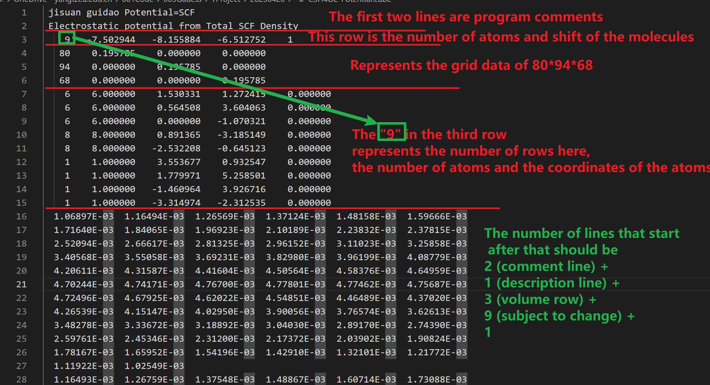
The following is a description of a typical cube file

Based on the above instructions, I wrote the following mathematica code：

(* === 1. File Name === *)

(* The name and location of the file to be read is specified here. *)

fileName = "https://dl-web.dropbox.com/s/aikd8iaxxvntifv/C3H4O2-Potential.cube";


(* === 2. Read All Lines === *)

(* Read all lines from the specified file. *)

lines = ReadList[fileName, String];



(* === 3. Comment Line === *)

(* Determine the line number for the comment line. *)

commentLine = 2;


(* === 4. Atom Count === *)

(* Determine the number of atoms and the line numbers where the atom coordinates are found. *)

atomNum = (lines[[3]] // StringSplit // ToExpression)[[1]];



(* === 5. Grid Size === *)

(* Determine the size of the grid and the line numbers where the grid dimensions are found. *)

gridLines = lines[[4 ;; 6]];
grid = ToExpression /@ StringSplit /@ gridLines;
gridSize = grid[[All, 1]];



(* === 6. Data Lines === *)

(* Determine the line numbers where the potential energy data starts and ends. *)

dataStart = 2 + 1 + 3 + atomNum + 1;
dataEnd = Length[lines];
dataLines = lines[[dataStart ;; dataEnd]];
data = Flatten[ToExpression /@ StringSplit /@ dataLines];


(* === 7. Potential Energy Data === *)

(* Reshape the potential energy data into a 3D array. *)

potentialData = ArrayReshape[data, gridSize];



(* === 8. Contour Plot === *)

(* Create a 3D contour plot of the potential energy data. *)

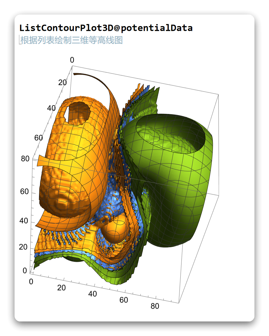
ListContourPlot3D@potentialData

The result was terrible, and then I used a different code：

minValue = Min[potentialData];
maxValue = Max[potentialData];

(*生成等值面级别列表*)
contourLevels = Range[minValue, maxValue, (maxValue - minValue)/20];

(*使用等值面级别列表绘制等值面图*)
ListContourPlot3D[potentialData, Contours -> contourLevels, 
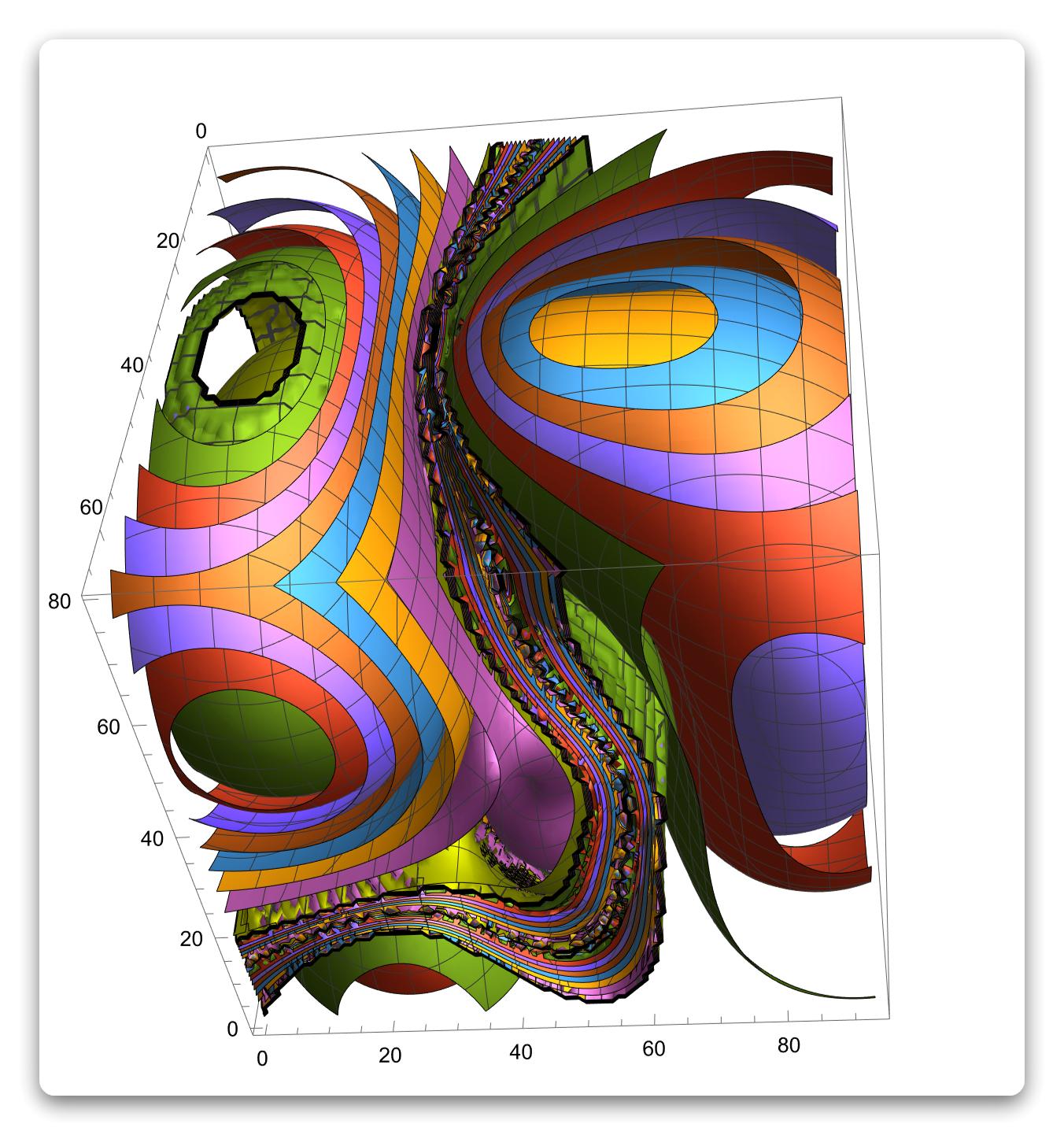
 PlotRange -> All]

It was still very bad, and then I changed my strategy

ListDensityPlot3D[potentialData, ColorFunction -> "TemperatureMap", 
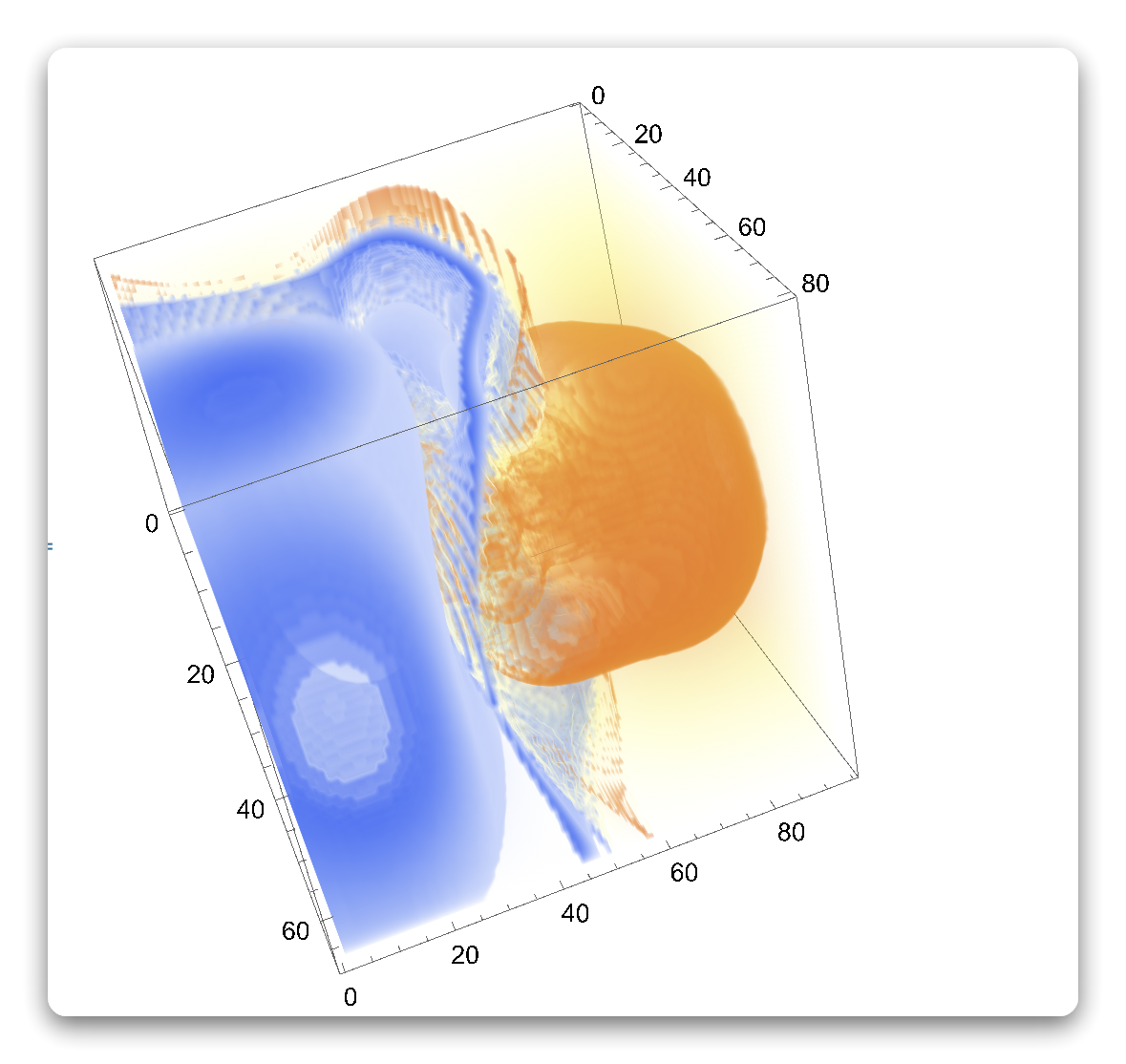
 PlotRange -> All]

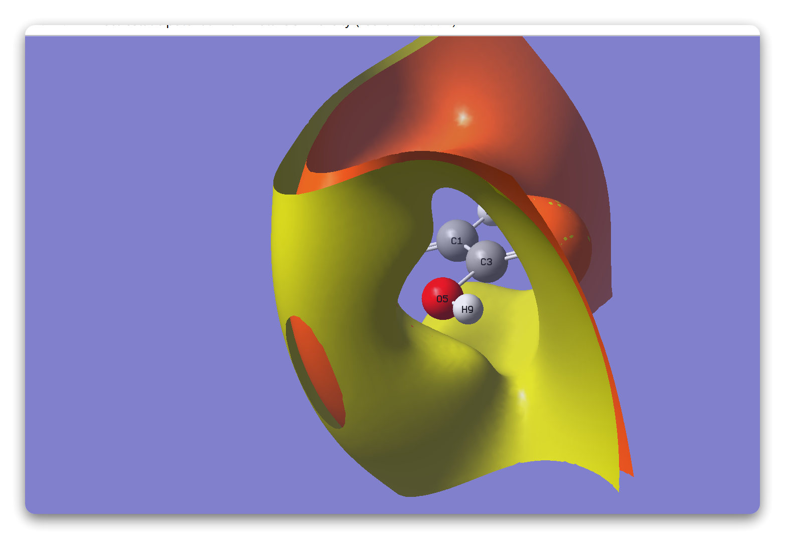
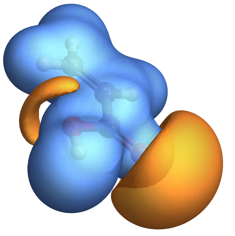
Looks much better, and much worse than gaussview produced

What can I do to match his performance, or even surpass his?

Answer 1

The first issue you are having is this:

In[262]:= ToExpression["1.06897E-03"]

Out[262]= -0.0942383

It's unfortunate, but that string is interpreted as a number times the constant E minus another number. I made the following adjustment to your code:

data = Flatten[ImportString[StringRiffle[dataLines, "\n"], "Table"]];
potentialData = Transpose[ArrayReshape[data, gridSize], 1 <-> 3]

and it plots nicely. I remembered the Transpose trick from the last time I wrote code like this.

In recent Mathematica versions you can get the plot directly through Import:

Import["/Users/jasonb/Downloads/C3H4O2-Potential.cube", "Graphics3D"]