45
$\begingroup$

Continuing with my interest on curvature of discrete surfaces here and here, I would like to also calculate and plot geodesics on discretised (triangulated) surfaces. Basically, my long-term idea would be to eventually estimate what path a particle would take if it is confined to a surface and moves at constant speed. There is one previous answer here, which goes along the lines of what I am looking for; however, it seems to be usable only for analytical surfaces (it gives the geodesics on a torus which is defined parametrically). I would interested if anyone has any ideas, hints or experience of how to do this, for arbitrary surfaces, and most importantly to use this in Mathematica?

One possibility would be to do it by numerically minimising the path between two points on a triangulated surface. An alternative would be to somehow use the surface curvatures (which we can now estimate) to rewrite the equations of motion of a particle.

The answers to this question have become a bit more involved and at the suggestion of user21 and J.M. I have split the answers up to make them easier to be found by anyone interested:

We have now 4 solutions implemented:

  1. "Out of the box" Dijkstra algorithm, quick and fast but limited to giving paths on edges of the surface.
  2. Exact LOS algorithm of (Balasubramanian, Polimeni and Schwartz), this is slow but calculates exact geodesics on the surface.
  3. Geodesics in Heat algorithm of (Crane, K., Weischedel, C., Wardetzky) (see also the fast implementation of Henrik Schumacher)
  4. A further implementation is the geodesic "shooter" from Henrik Schumacher here

Any further ideas or improvements in these codes would be most welcome. Other interesting algorithms to add to the list, could be the fast marching algorithm of Kimmel and Sethian or the MMP algorithm (exact algorithm) of Mitchell, Mount, and Papadimitriou.

$\endgroup$
24
  • 1
    $\begingroup$ Maybe of interest: Geodesics in heat $\endgroup$
    – user21
    Commented Mar 14, 2017 at 6:58
  • 2
    $\begingroup$ This came back to my attention today, after it was rather appropriately cited in a comment from this new question on MSE. I will add that this was one of my alll-time favorite threads; I up-voted the question and every response. Today I requested that response authors consider packaging and submitting their methods to the Wolfram Function Repository (@Szabolcs, this also applies to your method, if you can prise it free of IGraph internals). $\endgroup$ Commented Apr 19, 2020 at 16:47
  • 3
    $\begingroup$ If you have a version 11.x or greater (Not sure what value x takes), start with File > New > Repository Item > Function Repository Item. This will bring up a notebook with boilerplate with MyFunction in several key places. Just replace with actual code and documentation. Make liberal use of its Open Sample and Style Guidelines buttons. $\endgroup$ Commented Apr 19, 2020 at 17:33
  • 2
    $\begingroup$ @DanielLichtblau Thanks for the invitation! I could make it independent of IGraph/M in version 12.1, but I'm afraid the method is just not very good. The result depends too strongly on the mesh structure. It's a very, very rough approximation. $\endgroup$
    – Szabolcs
    Commented Apr 20, 2020 at 10:19
  • 1
    $\begingroup$ Sharp + Crane have a paper out this year with a very fast algorithm involving iterative edge flips: cs.cmu.edu/~kmcrane/Projects/FlipOut/FlipOut.pdf $\endgroup$
    – flinty
    Commented Nov 16, 2020 at 17:39

5 Answers 5

24
$\begingroup$

Nothing really new from my side. But since I really like the heat method and because the authors of the Geodesics-in-Heat paper are good friends of mine (Max Wardetzky is even my doctor father), here a slightly more performant implementation of the heat method.

solveHeat2[R_, a_, i_Integer] := Module[{delta, u, g, h, phi, n, sol, mass},
   sol = a[["HeatSolver"]];
   n = MeshCellCount[R, 0];
   delta = SparseArray[i -> 1., {n}, 0.];
   u = (a[["HeatSolver"]])[delta];
  If[NumericQ[a[["TotalTime"]]],
    mass = a[["Mass"]];
    u = Nest[sol[mass.#] &, u, Round[a[["TotalTime"]]/a[["StepSize"]]]];
    ];
   g = Partition[a[["Grad"]].u, 3];
   h = Flatten[-g/(Sqrt[Total[g^2, {2}]])];
   phi = (a[["LaplacianSolver"]])[a[["Div"]].h];
   phi - phi[[i]]
   ];

solveHeat2[R_, a_, i_?VectorQ] := 
  Module[{delta, u, g, h, phi, n, sol, mass}, 
   sol = a[["HeatSolver"]];
   n = MeshCellCount[R, 0];
   delta = SparseArray[Partition[i, 1] -> 1., {n}, 0.];
   u = (a[["HeatSolver"]])[delta];
   If[NumericQ[a[["TotalTime"]]], mass = a[["Mass"]];
    u = Nest[sol[mass . #] &, u, 
      Round[a[["TotalTime"]]/a[["StepSize"]]]];];
   g = Partition[a[["Grad"]] . u, 3];
   h = Flatten[-g/(Sqrt[Total[g^2, {2}]])];
   phi = (a[["LaplacianSolver"]])[a[["Div"]] . h];
   phi - Min[phi[[i]]]
   ];

heatDistprep2[R_, t_, T_: Automatic] := 
  Module[{pts, faces, areas, B, grad, div, mass, laplacian},
   pts = MeshCoordinates[R];
   faces = MeshCells[R, 2, "Multicells" -> True][[1, 1]];
   areas = PropertyValue[{R, 2}, MeshCellMeasure];
   B = With[{n = Length[pts], m = Length[faces]},
     Transpose[SparseArray @@ {Automatic, {3 m, n}, 0,
        {1, {Range[0, 3 m], Partition[Flatten[faces], 1]},
         ConstantArray[1, 3 m]}}]];
   grad = Transpose[Dot[B,
      With[{blocks = getFaceHeightInverseVectors3D[ Partition[pts[[Flatten[faces]]], 3]]},
       SparseArray @@ {Automatic, #1 {##2}, 0.,
           {1, {Range[0, 1 ##, #3], getSparseDiagonalBlockMatrixSimplePattern[##]}, 
            Flatten[blocks]
            }} & @@ Dimensions[blocks]]]];
   div = Transpose[
     Times[SparseArray[Flatten[Transpose[ConstantArray[areas, 3]]]], 
      grad]];
   mass = Dot[B,
     Dot[
      With[{blocks = areas ConstantArray[ 
          N[{{1/6, 1/12, 1/12}, {1/12, 1/6, 1/12}, {1/12, 1/12, 1/6}}], Length[faces]]
         },
        SparseArray @@ {Automatic, #1 {##2}, 0.,
            {1, {Range[0, 1 ##, #3], getSparseDiagonalBlockMatrixSimplePattern[##]}, 
             Flatten[blocks]}
            } & @@ Dimensions[blocks]
        ].Transpose[B]
      ]
     ];
   laplacian = div.grad;
   Association[
    "Laplacian" -> laplacian, "Div" -> div, "Grad" -> grad, 
    "Mass" -> mass,
    "LaplacianSolver" -> LinearSolve[laplacian, "Method" -> "Pardiso"],
    "HeatSolver" -> LinearSolve[mass + t laplacian, "Method" -> "Pardiso"], "StepSize" -> t, "TotalTime" -> T
    ]
   ];

Block[{PP, P, h, heightvectors, t, l},
  PP = Table[Compile`GetElement[P, i, j], {i, 1, 3}, {j, 1, 3}];
  h = {
    (PP[[1]] - (1 - t) PP[[2]] - t PP[[3]]),
    (PP[[2]] - (1 - t) PP[[3]] - t PP[[1]]),
    (PP[[3]] - (1 - t) PP[[1]] - t PP[[2]])
    };
  l = {(PP[[3]] - PP[[2]]), (PP[[1]] - PP[[3]]), (PP[[2]] - PP[[1]])};
  heightvectors = Table[Together[h[[i]] /. Solve[h[[i]].l[[i]] == 0, t][[1]]], {i, 1, 3}];
  
  getFaceHeightInverseVectors3D = 
   With[{code = heightvectors/Total[heightvectors^2, {2}]},
    Compile[{{P, _Real, 2}},
     code,
     CompilationTarget -> "C",
     RuntimeAttributes -> {Listable},
     Parallelization -> True,
     RuntimeOptions -> "Speed"
     ]
    ]
  ];

getSparseDiagonalBlockMatrixSimplePattern = 
  Compile[{{b, _Integer}, {h, _Integer}, {w, _Integer}}, 
   Partition[Flatten@Table[k + i w, {i, 0, b - 1}, {j, h}, {k, w}], 1],
   CompilationTarget -> "C", RuntimeOptions -> "Speed"];

plot[R_, ϕ_] := 
 Module[{colfun, i, numlevels, res, width, contouropac, opac, tex, θ, h, n, contourcol, a, c},
  colfun = ColorData["DarkRainbow"];
  i = 1;
  numlevels = 100;
  res = 1024;
  width = 11;
  contouropac = 1.;
  opac = 1.;
  tex = If[numlevels > 1,
    θ = 2;
    h = Ceiling[res/numlevels];
    n = numlevels h + θ (numlevels + 1);
    contourcol = N[{0, 0, 0, 1}];
    contourcol[[4]] = N[contouropac];
    a = Join[
      Developer`ToPackedArray[N[List @@@ (colfun) /@ (Subdivide[1., 0., n - 1])]],
      ConstantArray[N[opac], {n, 1}],
      2
      ];
    a = Transpose[Developer`ToPackedArray[{a}[[ConstantArray[1, width + 2]]]]];
    a[[Join @@ 
       Table[Range[
         1 + i (h + θ), θ + i (h + θ)], {i, 0, 
         numlevels}], All]] = contourcol;
    a[[All, 1 ;; 1]] = contourcol;
    a[[All, -1 ;; -1]] = contourcol;
    Image[a, ColorSpace -> "RGB"]
    ,
    n = res;
    a = Transpose[Developer`ToPackedArray[
       {List @@@ (colfun /@ (Subdivide[1., 0., n - 1]))}[[
        ConstantArray[1, width]]]
       ]];
    Image[a, ColorSpace -> "RGB"]
    ];
  c = Rescale[-ϕ];
  Graphics3D[{EdgeForm[], Texture[tex], Specularity[White, 30],
    GraphicsComplex[
     MeshCoordinates[R],
     MeshCells[R, 2, "Multicells" -> True],
     VertexNormals -> Region`Mesh`MeshCellNormals[R, 0],
     VertexTextureCoordinates -> 
      Transpose[{ConstantArray[0.5, Length[c]], c}]
     ]
    },
   Boxed -> False,
   Lighting -> "Neutral"
   ]
  ];

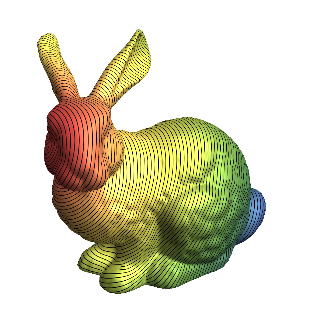
Usage and test:

R = ExampleData[{"Geometry3D", "StanfordBunny"}, "MeshRegion"];
data = heatDistprep2[R, 0.01]; // AbsoluteTiming // First
ϕ = solveHeat2[R, data, 1]; // AbsoluteTiming // First

0.374875

0.040334

In this implementation, data contains already the factorized matrices (for the heat method, a fixed time step size has to be submitted to heatDistprep2).

Plotting can be done also more efficiently with

plot[R, ϕ]

enter image description here

#Remarks

There is more fine-tuning to be done. Keenan and Max told me that this method performs really good only if the surface triangulation is an intrinsic Delaunay triangulation. This can always be achieved starting from a given triangle mesh by several edge flips (i.e., replacing the edge between two triangles by the other diagonal of the quad formed by the two triangles). Moreover, the time step size t for the heat equation step should decrease with the maximal radius h of the triangles; somehow like $t = \frac{h^2}{2}$ IIRC.

$\endgroup$
14
  • 1
    $\begingroup$ Thanks for the flowers. For the meaning of the SparseArray@@{...} syntax which allows for very fast matrix construction, see this post. $\endgroup$ Commented Jun 19, 2018 at 6:37
  • 1
    $\begingroup$ Really wonderful work! I wonder if this is something for WFR. FYI "Multicells" -> True seems to be outdated. I also get an error CCompilerDriverCreateLibrary::cmperr: Compile error: xcrun: error: invalid active developer path (/Library/Developer/CommandLineTools), missing xcrun at: /Library/Developer/CommandLineTools/usr/bin/xcrun` $\endgroup$ Commented Feb 20, 2020 at 4:51
  • 2
    $\begingroup$ Hm. Maybe. I don't know whether I find the time to flesh this out for WFR. Towards "Multicells": This option is just undocumented; user21 told me about that. It is so super secret that even Mathematica herself does not know of its existence. This can be fixed with Unprotect[MeshCells]; SyntaxInformation[MeshCells] = {"ArgumentsPattern" -> {_, _, OptionsPattern[]}}; Protect[MeshCells]; I think this option is so crucial for working efficiently with MeshRegions that it should be documented as soon as possible. And I hope that it won't be outdated with the upcoming release... $\endgroup$ Commented Feb 20, 2020 at 6:43
  • 1
    $\begingroup$ About the compilation problems: I do not think that I can do anything about that; this must be something specific to your installation. It runs for me nicely. $\endgroup$ Commented Feb 20, 2020 at 6:44
  • 1
    $\begingroup$ @DanielLichtblau I'd love to, but there is so much else to do... =/ $\endgroup$ Commented Apr 19, 2020 at 18:07
36
+100
$\begingroup$

Geodesics in Heat Algorithm

At the suggestion of @user21 I am splitting up my answers to help make the code(s) for calculating geodesics distances easier to find for other people interested in these sorts of algorithms.

The Geodesics in Heat algorithm is a fast approximate algorithm for estimating geodesic distances on discrete meshes (but also a variety of other discrete systems i.e. point clouds etc). See (Crane, K., Weischedel, C., Wardetzky, M. ACM Transactions on Graphics 2013) for a link to the paper. The paper describes the algorithm very well, but I will attempt to give a simplified description. Basically the algorithm uses the idea that heat diffusing from a given point on a surface will follow shortest distances on the surface. Therefore if one can simulate heat diffusion on the mesh, then the local heat gradients should point in the direction of the heat source. These can then be used (with the Poisson equation) to solve for distances to the source at each point on the mesh. In principle any discrete set of objects can be used as long as gradient, divergence and Laplace operators can be defined.

For the following I followed the matlab implementation on G. Peyré's website, Numerical Tours, which gives a whole range of useful examples of graph algorithms. In principle the matlab toolboxes posted there could also be used via Matlink but for the sake of understanding (and the cost of a Matlab licence) I wanted to code this in Mathematica. Thanks especially to G. Peyré for his implementation and permission to post this code and a link to his site.

The algorithm follows the following steps (Steps taken from the paper):

  1. Integrate the equation $\dot{u} = \Delta u$ for a fixed time, $t$
  2. Evaluate the vector field at each point on the mesh: $X = -\nabla u/|\nabla u|$
  3. Solve the Poisson equation $\Delta \phi = \nabla . X $

This I implemented in the following modules:

The code is as follows:

Pre-calculating values on a given mesh:

heatDistprep[mesh0_] := Module[{a = mesh0, vertices, nvertices, edges, edgelengths, nedges, faces, faceareas, unnormfacenormals, acalc, facesnormals, facecenters, nfaces, oppedgevect, wi1, wi2, wi3, sumAr1, sumAr2, sumAr3, areaar, gradmat1, gradmat2, gradmat3, gradOp, arear2, divMat, divOp, Delta, t1, t2, t3, t4, t5, , Ac, ct, wc, deltacot, vertexcoordtrips, adjMat},
vertices = MeshCoordinates[a]; (*List of vertices*)
edges = MeshCells[a, 1] /. Line[p_] :> p; (*List of edges*)
faces = MeshCells[a, 2] /. Polygon[p_] :> p; (*List of faces*)
nvertices = Length[vertices];
nedges = Length[edges];
nfaces = Length[faces];
adjMat = SparseArray[Join[({#1, #2} -> 1) & @@@ edges, ({#2, #1} -> 1) & @@@edges]]; (*Adjacency Matrix for vertices*)
edgelengths = PropertyValue[{a, 1}, MeshCellMeasure];
faceareas = PropertyValue[{a, 2}, MeshCellMeasure];
vertexcoordtrips = Map[vertices[[#]] &, faces];
unnormfacenormals = Cross[#3 - #2, #1 - #2] & @@@ vertexcoordtrips;
acalc = (Norm /@ unnormfacenormals)/2;
facesnormals = Normalize /@ unnormfacenormals;
facecenters = Total[{#1, #2, #3}]/3 & @@@ vertexcoordtrips;
oppedgevect = (#1 - #2) & @@@ Partition[#, 2, 1, 3] & /@vertexcoordtrips;
wi1 = -Cross[oppedgevect[[#, 1]], facesnormals[[#]]] & /@Range[nfaces];
wi2 = -Cross[oppedgevect[[#, 2]], facesnormals[[#]]] & /@Range[nfaces];
wi3 = -Cross[oppedgevect[[#, 3]], facesnormals[[#]]] & /@Range[nfaces];
sumAr1 = SparseArray[Join[Map[{#, faces[[#, 1]]} -> wi1[[#, 1]] &, Range[nfaces]],Map[{#, faces[[#, 2]]} -> wi2[[#, 1]] &, Range[nfaces]],Map[{#, faces[[#, 3]]} -> wi3[[#, 1]] &, Range[nfaces]]]];
sumAr2 = SparseArray[Join[Map[{#, faces[[#, 1]]} -> wi1[[#, 2]] &, Range[nfaces]], Map[{#, faces[[#, 2]]} -> wi2[[#, 2]] &, Range[nfaces]],Map[{#, faces[[#, 3]]} -> wi3[[#, 2]] &, Range[nfaces]]]];
sumAr3 =SparseArray[Join[Map[{#, faces[[#, 1]]} -> wi1[[#, 3]] &, Range[nfaces]], Map[{#, faces[[#, 2]]} -> wi2[[#, 3]] &, Range[nfaces]], Map[{#, faces[[#, 3]]} -> wi3[[#, 3]] &, Range[nfaces]]]];
areaar = SparseArray[Table[{i, i} -> 1/(2*acalc[[i]]), {i, nfaces}]];
gradmat1 = areaar.sumAr1;
gradmat2 = areaar.sumAr2;
gradmat3 = areaar.sumAr3;
gradOp[u_] := Transpose[{gradmat1.u, gradmat2.u, gradmat3.u}];
arear2 = SparseArray[Table[{i, i} -> (2*faceareas[[i]]), {i, nfaces}]];
divMat = {Transpose[gradmat1].arear2, Transpose[gradmat2].arear2,Transpose[gradmat3].arear2};
divOp[q_] := divMat[[1]].q[[All, 1]] + divMat[[2]].q[[All, 2]] + divMat[[3]].q[[All, 3]];
Delta = divMat[[1]].gradmat1 + divMat[[2]].gradmat2 + divMat[[3]].gradmat3;
SetSystemOptions["SparseArrayOptions" -> {"TreatRepeatedEntries" -> 1}]; (*Required to allow addition of value assignment to Sparse Array*)
t1 = Join[faces[[All, 1]], faces[[All, 2]], faces[[All, 3]]];
t2 = Join[acalc, acalc, acalc];
Ac = SparseArray[Table[{t1[[i]], t1[[i]]} -> t2[[i]], {i, nfaces*3}]];
SetSystemOptions["SparseArrayOptions" -> {"TreatRepeatedEntries" -> 0}];
{Ac, Delta, gradOp, divOp, nvertices, vertices, adjMat}
]

Solving the equation

solveHeat[mesh0_, prepvals_, i0_, t0_] := Module[{nvertices, delta, t, u, Ac, Delta, g, h, phi, gradOp, divOp, vertices, plotdata},
vertices = prepvals[[6]];
nvertices = prepvals[[5]];
Ac = prepvals[[1]];
Delta = prepvals[[2]];
gradOp = prepvals[[3]];
divOp = prepvals[[4]];
delta = Table[If[i == i0, 1, 0], {i, nvertices}];
t = t0;
u = LinearSolve[(Ac + t*Delta), delta];
g = gradOp[u];
h = -Normalize /@ g;
phi = LinearSolve[Delta, divOp[h]];
plotdata = Map[Join[vertices[[#]], {phi[[#]]}] &, Range[Length[vertices]]];

{ListSliceContourPlot3D[plotdata, a, ContourShading -> Automatic, ColorFunction -> "BrightBands", Boxed -> False, Axes -> False],phi}
] 

Using the answer of Jason B. here we can plot the results of such a calculation using the following:

a = BoundaryDiscretizeRegion[ImplicitRegion[((Sqrt[x^2 + y^2] - 2)/0.8)^2 + z^2 <= 1, {x, y, z}], MaxCellMeasure -> {"Length" -> 0.2}];
test = heatDistprep[a];
solveHeat[a, test, 10, 0.1]

giving:

geodesics heat on torus

I have implemented a "rough algorithm" to calculate the minimal path between two points (along edges). This process first uses the geodesics in heat algorithm to solve for distances to a point $i$ on the surfaces everywhere. Then upon picking another point $j$ it calculates the chain of intermediate vertices such that the distance is always decreasing. As this gives a path that travels along edges, it is not unique and perhaps should be combined with a more exact algorithm to allow the path to go over the faces.

pathHeat[mesh0_, meshdata_, iend_, istart_] := Module[{phi, edges, adjMat, phi0, neighlist, vallist, i, j, vlist, vertices, pathline},
phi = solveHeat[mesh0, meshdata, iend, 0.5][[1]];
adjMat = meshdata[[7]];
vlist = {istart};
i = istart;
While[i != iend, 
   neighlist = Flatten[adjMat[[i]]["NonzeroPositions"]];
   vallist = (phi[[#]] & /@ neighlist);
   j = Ordering[vallist, 1][[1]]; (*Choose smallest distance*)
   AppendTo[vlist, neighlist[[j]]];
   i = neighlist[[j]];
];
vlist = Flatten[vlist];
vertices = meshdata[[6]];
pathline = vertices[[#]] & /@ vlist;
{vlist, pathline}
];

To test this I used the "Standford Bunny" from the `3DGraphics' examples in Mathematica. This is pretty quick.

a = DiscretizeGraphics[ExampleData[{"Geometry3D", "StanfordBunny"}]];
test = heatDistprep[a];
test2 = pathHeat[a, test, 300, 1700];
phi = solveHeat[a, test, 300, 0.5][[1]];
vertices = test[[6]];
plotdata = Map[Join[vertices[[#]], {phi[[#]]}] &, Range[Length[vertices]]];
cplot = ListSliceContourPlot3D[plotdata, a, ContourShading -> Automatic, ColorFunction -> "BrightBands",  Boxed -> False, Axes -> False];
pathplot = Graphics3D[{Red, Thick, Line[test2[[2]]]}];
Show[cplot, pathplot]

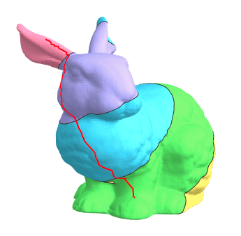
which gives the following as output in about 80 seconds (I haven't tried this with the LOS algorithm yet):

bunny path

I hope someone may find this useful.

$\endgroup$
6
  • 4
    $\begingroup$ Awesome answer! Just for anyone who is interested in more background info for the algorithm, Keenan Crane has some very nicely narrated videos that explain the details and motivation of the algorithm on his Youtube channel, e.g. this one and a broader talk, that covers three topics. $\endgroup$ Commented Mar 22, 2017 at 13:05
  • 1
    $\begingroup$ Very nice. You could send Keenan Crane a note about your implementation, I am sure he would appreciate that. $\endgroup$
    – user21
    Commented Mar 23, 2017 at 8:14
  • $\begingroup$ @user21 I will do. Thanks for letting me know about the algorithm in the first place. Haven't yet got the fast marching working, but hopefully I will get around to it. Would be nice to be able to compare different algorithms in the one system. $\endgroup$
    – Dunlop
    Commented Mar 23, 2017 at 8:22
  • $\begingroup$ This is nice. If I find time, I'll see if I can optimize this implementation a bit further. (I was also looking into biharmonic distance before this, but Crane et al. note that it has shortcomings compared to this approach.) $\endgroup$ Commented Mar 23, 2017 at 9:18
  • 1
    $\begingroup$ @user21 Thanks for the bounty but to be honest thanks much more for the hint about the algorithm. The more I read the more powerful it seems, especially if one can generalise it to point clouds etc. Will see if I can expand this answer if I get some more time. $\endgroup$
    – Dunlop
    Commented Mar 28, 2017 at 19:57
18
$\begingroup$

Here is an exact algorithm but heavier to implement and to optimise. I chose to implement the "Line of Sight Algorithm" from Balasubramanian, Polimeni and Schwartz (REF).

Exact Line of Sight algorithm

An algorithm which calculates the exact distance on polyhedral surfaces is the algorithm proposed by Balasubramanian, Polimeni and Schwartz (REF). They call this the Line of Sight (LOS) algorithm. For me this was one of the easier exact algorithms to implement although it requires lots of book keeping, and is rather slow at least in my implementation. (Any ideas for speeding this up or dealing with book keeping and memory usage are welcome). The idea behind this algorithm is rather simple. It relies on the observation that a geodesic on a triangulated surface must consist of straight lines when passing over the faces, these lines only change direction when passing over edges (vertices). Furthermore if one takes the set of triangles that a given geodesic passes through on the 3D surface, and then “unfolds” them so that all these triangles are contained in a flat plane (2D), then the geodesic must then be a straight line. As a consequence what one can do is to calculate “all” possible unfoldings of “all” chains of connected triangles on a surface, and then calculate the distance in 2D. Perhaps not the clearest description, but please look at the paper for a more detailed description of the algorithm (REF). It must be stated that this (and the Dijkstra) like implementation calculates shortest distances (or estimates) between vertices.

The algorithm is not fast in my implementation, however once the shortest distance map is created for a given mesh, the shortest path calculations are pretty quick.

I tested this based on the mesh produced here:

dodeq = z^6 - 5 (x^2 + y^2) z^4 + 5 (x^2 + y^2)^2 z^2 - 
   2 (x^4 - 10 x^2 y^2 + 5 y^4) x z + (x^2 + y^2 + z^2)^3 - (x^2 + 
      y^2 + z^2)^2 + (x^2 + y^2 + z^2) - 1;
dodeqmesh02 = 
  BoundaryDiscretizeRegion[ImplicitRegion[dodeq <= 0, {x, y, z}], 
   MaxCellMeasure -> {"Length" -> 0.2}];
a = dodeqmesh02

which has 916 vertices. Total running time was a couple of hours…

The resultant minimal path between 2 vertices and the colour coded distance map (scaled from 0 to 1) is shown here:
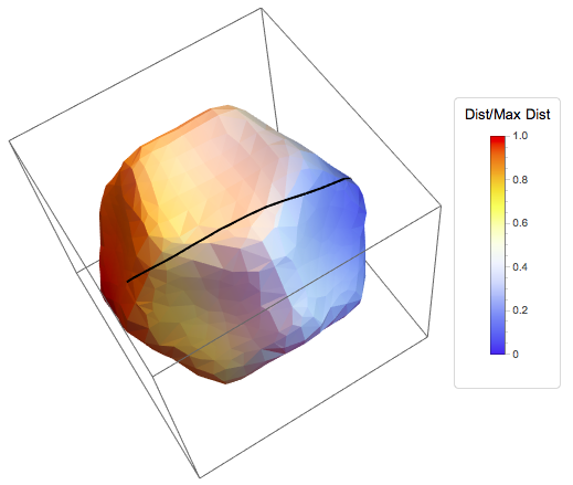
sample shortest path

The code for the algorithm I will give at the end of this post as well as the code for the plotting. I am sure this can be sped up (I am trying to work out a way to compile this efficiently), and perhaps there is some reduncancy in the code, but for those interested it could be useful to compare with other algorithms. Any suggestions would be most welcome. There are other algorithms that I also will try to implement, but most likely it could be a while before I get to this stage.

Line of Sight Algorithm Code

losAlgorithm[mesh_] := 
  Module[{mesh0 = mesh, pts, nvertices, edges, tri, va, edgelengths, 
    distMatrix, tchainlists, Δθprec, vtrilist, 
    ntri, tl3dstore, tnum, eAB, vA, vB, vD, vS, e1, e2, el, 
    vertmeshlabels, vertex2Dcoords, trilist2D, trichain3Dlabels, 
    trilabel, trilabel0, coordsA, coordsB, coordsD, 
    ang, θ, θmin, θmax, vnum2D, tchainstack, 
    doubletri, boundaryEdgeQ, tpop, trichainnum, vectAB, angAB, 
    angBAD, e3, el3, δSD, outMatrix, θMatrix, tMatrix, 
    distMatrixsym},
   (**************************)
   (*Numerical Parameters*)
   (**************************)      
   dthetaprec =  0.05; (*Precision in Theta max - Theta min , 
   perhaps can be removed at somestage but at the moment useful for testing*) 
   (**************************)
   (*Mesh Calculations*)
   (**************************)

   (*List of coordinates of all vertices on the mesh*)

   pts = MeshCoordinates[mesh];
   (*Number of vertices on the mesh*)
   nvertices = Length[pts];
   (*List of all edges on the mesh, 
   in terms of pairs of vertex indices*)

   edges = MeshCells[mesh, 1] /. Line[p_] :> p ;
   (*List of the "ordered" vertex index triples for all triangles on the mesh*)
   tri = MeshCells[mesh, 2] /. Polygon[p_] :> p; 
   (*List of edgelengths numbered by edge *)

   edgelengths = PropertyValue[{mesh, 1}, MeshCellMeasure];
   (*List of the angles within each of the corners of all triangles on the mesh*)

   va = VectorAngle[#1 - #2, #3 - #2] & @@@ 
       Partition[#, 3, 1, {2, -2}] & /@ 
     MeshPrimitives[mesh, {2}][[All, 1]];

   (**************************)
   (*Preparation of data structures for storage*)
   (**************************)
   (*Matrix to store all distances between all pairs of vertices*)

   distMatrix = 
    Table[If[i == j, 0], {i, 1, nvertices}, {j, 1, nvertices}];
   (*Matrix to store all angles between pairs of vertices*)

   ThetaMatrix = 
    Table[If[i == j, 0], {i, 1, nvertices}, {j, 1, nvertices}];
   (*Matrix to store all triangle chains (in 3D labelling) between pairs of vertices*)

   tMatrix = 
    Table[If[i == j, 0], {i, 1, nvertices}, {j, 1, nvertices}];

   (**************************)
   (*Start of Algorithm*)
   (**************************)

   (********)
   (*Step 1 - 
   Choose a vertex vS on the mesh (Here we map over all Vertices) *)

   (********)
   Do[
    (********)
    (*Step 2 - 
    Choose a triangle containing vS as a vertex*)
    (********)

   (*Create a list of triangles around the vertex vS*)

    vtrilist = Position[tri, vS];
    (*Number of triangles around vertex S*)

    ntri = Length[vtrilist];
    (*Choose the first triangle in the list*)
    tnum = 1;
    (*While Loop to be performed over all triangles around vertex S*)
    (**********************)
    (******
    while loop here******)
    (**********************)

    While[tnum < ntri,
     Label[step2];
     If[tnum == ntri + 1, Break[]];
     (*Calculate ordered list of vertices A and B assuming we have outward oriented facets*)

     eAB = tri[[
        vtrilist[[tnum]][[1]]]] /. {vS, a_, b_} | {b_, vS, a_} | {a_, b_, vS} :> {a, b};
     vA = eAB[[1]]; (*Set vertex A*)
     vB = eAB[[2]]; (*Set vertex B*)
     (*Calculate labels of the vertices of first two edges*)
     e1 = {vA, vS};
     e2 = {vB, vS};
     (*Calculate edge lengths for the first triangle in the chain(s)*)

          el = edgelengths[[Join[Flatten[Position[edges, e1 | Reverse[e1]]],Flatten[Position[edges, e2 | Reverse[e2]]]]]];
     (*Store the edge length data in the distance matrix*)

     distMatrix[[vS, vA]] = el[[1]];
     distMatrix[[vS, vB]] = el[[2]];
     (*Create a set of (temporary) lists which will hold information about vertexlabels, 
     coordinates etc*)
     (*Lists will be stored (perhaps in tMatrix etc), 
     whenever a new triangle chain is created*)
     (*Probably this information is not needed in the final algorithm, 
     but will be needed for debugging*)

     (*List of the vertex labels from the original mesh in the triangle chain*)
     vertmeshlabels = {}; 
     (*List of the 2D transformed coordinates of the vertices*)

     vertex2Dcoords = {}; 
     (*List of the vertex triples that make up each flattened triangle chain in 2D*)
     trilist2D = {}; 
     (*List of 3D face triangle labels from the mesh in the triangle chain*)

     trichain3Dlabels = {};
     (*label of current triangle in the triangle chain *)

     trilabel = vtrilist[[tnum]][[1]]; 
     (*Set previous triangle label to the current one (used for later calculations) *)
     trilabel0 = trilabel;
     (*Add the first triangle label to the list of 3D triangle(face) labels in the chain*)

     trichain3Dlabels = {trichain3Dlabels, trilabel};
     (*Map first triangle in the chain to the plane*)
     (*Origin Vertex vS*)
     (*Add vS mesh label to list*)

     vertmeshlabels = {vertmeshlabels, vS};
     (*Add vS 2D coordinate pair to 2D coordinate list*)

     vertex2Dcoords = {vertex2Dcoords, {0, 0}};
     (*Vertex vA *)
     (*Add vA mesh label to list*)

     vertmeshlabels = {vertmeshlabels, vA};
     coordsA = {el[[1]], 0};  (*Calculate 2D flattened coordinates of vertex vA*)

     (*Add vA 2D coordinate pair to 2D coordinate list*)

     vertex2Dcoords = {vertex2Dcoords, coordsA};
     (*Vertex vB *)
     (*Add vB mesh label to list*)

     vertmeshlabels = {vertmeshlabels, vB};
     ang = va[[vtrilist[[tnum]][[1]], vtrilist[[tnum]][[2]]]];
     coordsB = {el[[2]]*Cos[ang], el[[2]]*Sin[ang]}; (*Calculate 2D flattened coordinates of vertex vB*)

     (*Add vB 2D coordinate pair to 2D coordinate list*)

     vertex2Dcoords = {vertex2Dcoords, coordsB};
     (*Add the ordered triple of vertices to the 2D triangle list*)

        trilist2D = {trilist2D, {1, 2, 3}};
     thetamin = 0; (*Set min angle to be 0*)
     thetamax = ang; (*Set max angle to be the angle <BSA*)

     (********)
     (*Step 3*)
     (********)
     (*Counter of number of 2D vertices in triangle chain, will be reset everytime we do a new chain? starts at vertex 4*)

     vnum2D = 4;
     (*Initialise chain stack to enable chain branching, this first starts off as being empty*)
     (*What we also want to do is to rebuild a new chain stack for each branch *)

     tchainstack = {};
     (********)
     (*Step 4*)
     (********)

     doubletri = 0; (*Label = 0 if triangles not repeated in chain, = 1 if repeated*)

     nextensions = 1; (*Max number of extensions of triangle chain within one chain*)
     While[nextensions < 10000,
      Label[step4];
      (*BoundaryQ - Returns False if edge NOT a boundary, 
      True only 1 tri is attached to  edge vA -> vB*)

      boundaryEdgeQ = Intersection[Position[tri, vA][[All, 1]], Position[tri, vB][[All, 1]]] != 2; 
      (*Calculate whether we are within machine precision or not \
thetamax-thetamin< dthetaprec*)

      If[(thetamax - thetamin < dthetaprec) || 
        boundaryEdgeQ || (doubletri == 1),
       If[(tchainstack == {}),
         tnum++;
         Goto[step2],(*picknewtriangle*)
         {tpop, tchainstack} = {#, {##2}} & @@ tchainstack;
         (*newstructure of tchainstack*)

         tchainstack = tchainstack[[1]];
         (*to reset values so that we go down other chains*)
         (*Tlabel, Alabel, Blabel, coordsA2D,coordsB2D,thetamin,thetamax*)
         trilabel0 = tpop[[1]];
         vA = tpop[[2]];
         vB = tpop[[3]];
         coordsA = tpop[[4]];
         coordsB = tpop[[5]];
         thetamin = tpop[[6]];
         thetamax = tpop[[7]];
         vnum2D = tpop[[8]];
         (*here we store the previous tchainlist for plotting*)

         vertmeshlabels =  Flatten[vertmeshlabels]; (*Flatten the linked list created previously*)

         trichain3Dlabels = Flatten[trichain3Dlabels];(*Flatten the linked list created previously*)

         vertex2Dcoords = Partition[Flatten[vertex2Dcoords],2];(*Flatten the linked list created previously*)

         trilist2D = 
          Partition[Flatten[trilist2D], 3];(*Flatten the linked list created previously*)
         (*now we need to go back in the list and "restart" so to say the counters*)
         (*need to reset the storage, and also the vnum2D otherwise we wont have diff chains, mainly important for plotting, but probably stops labelling effects*)

         trichainnum = Position[trichain3Dlabels, trilabel0][[1, 1]];
         trichain3Dlabels = Take[trichain3Dlabels, trichainnum];
         vertmeshlabels = Take[vertmeshlabels, vnum2D - 1];
         trilist2D = Take[trilist2D, trichainnum];
         vertex2Dcoords = Take[vertex2Dcoords, vnum2D - 1];
         (*Reset doubled triangle label to zero *)

         doubletri = 0; 
         ];
       ];

      (*Find triangle label on the other side of the edge AB on the previous triangle in the chain*)

      trilabel = Select[Intersection[Position[tri, vA][[All, 1]],Position[tri, vB][[All, 1]]], # != trilabel0 &][[1]];
      (*Check to see if triangle has been visited before in the chain if yes, go to new chainstack,*)

      If[MemberQ[trichain3Dlabels, trilabel], doubletri = 1; 
       Goto[step4];];
      trilabel0 = trilabel;
      (********)
      (*Step 5*)
      (********)
      (*Add the 3D triangle label to the triangle chain list*)

      trichain3Dlabels = {trichain3Dlabels, trilabel};
      (*Calculate the label of the next vertex*)

      vD = Select[tri[[trilabel]], False == MemberQ[{vA, vB}, #] &][[1]];
      vertmeshlabels = {vertmeshlabels, vD};
      (*Calculate angle, in 2D, of edge A-B, wrt x-axis*)

      vectAB = coordsB - coordsA;
      angAB = ArcTan[vectAB[[1]], vectAB[[2]]];
      (*Calculate angle <BAD*)

      angBAD = va[[trilabel, Position[tri[[trilabel]], vA][[1, 1]]]];
      e3 = {vA, vD};
      el3 = edgelengths[[Flatten[Position[edges, e3 | Reverse[e3]]]]][[1]];
      (*Calculation of 2D flattened coordinates of vertex D*)

      coordsD = (coordsA + {el3*Cos[angAB - angBAD], el3*Sin[angAB - angBAD]});
      vertex2Dcoords = {vertex2Dcoords, coordsD};
      (*Add ordered triple of vertices to triangle list*)

      trilist2D = {trilist2D, Flatten[Map[Position[vertmeshlabels, #] &,tri[[trilabel]]]]};
      (*Increment  vnum2D*)
      vnum2D = vnum2D + 1;
      (*Calculate the angle that SD makes with the x-axis*)
      theta = ArcTan[coordsD[[1]], coordsD[[2]]]; 
      (********)
      (*Step 6 - If theta<thetamin set A = D and return to step 4*)
      (********)

      If[theta < thetamin,
       vA = vD;
       coordsA = coordsD;
       Goto[step4];
       ];
      (********)
      (*Step 7 - If theta>thetamax set B =  D and return to step 4*)
      (********)

      If[theta > thetamax,
       vB = vD;
       coordsB = coordsD;
       Goto[step4];
       ];
      (********)
      (*Step 8 - 
      If theta is an element (thetamin,thetamax)*)
      (********)
      (*Compute Euclidean distance between planar representations of S and D*)
      deltaSD = Sqrt[Total[coordsD^2]];
      (*Update distance matrix and angle matrix if the calculated distance is smaller than what was previously stored*)

      If[distMatrix[[vS, vD]] == Null,
       distMatrix[[vS, vD]] = deltaSD;
       thetaMatrix[[vS, vD]] = theta;
       tMatrix[[vS, vD]] = Flatten[trichain3Dlabels],
       If[distMatrix[[vS, vD]] > deltaSD,
        distMatrix[[vS, vD]] = deltaSD;
        thetaMatrix[[vS, vD]] = theta;
        tMatrix[[vS, vD]] = Flatten[trichain3Dlabels]
        ]];
      (*Store information needed to extend triangle over AD onto stack: Tlabel, Alabel, Blabel, coordsA2D,coordsB2D,thetamin,thetamax*)

      tchainstack = {{trilabel, vA, vD, coordsA, coordsD, thetamin, thetamax, vnum2D}, tchainstack};
      (*Extend triangle chain over edge BD, set A = D and set thetamin = theta*)
      vA = vD;
      coordsA = coordsD;
      thetamin = theta;
      nextensions++;
      ];
     ], {vS, nvertices}
    ];
   (*Now make sure distance matrix is symmetric and replace Null by large number, Infinity in this case *)

   distMatrixsym = Table[Min[{distMatrix[[i, j]] /. Null -> Infinity, 
       distMatrix[[j, i]] /. Null -> Infinity}], {i, 1, nvertices}, {j, 1, nvertices}];
   distMatrix = distMatrix /. Null -> Infinity;
   (*Implement shortest distance *)

   outMatrix =  GraphDistanceMatrix[WeightedAdjacencyGraph[distMatrixsym],Method -> "FloydWarshall"];
   {outMatrix, tri, thetaMatrix, tMatrix, distMatrixsym, distMatrix}
   ];

LOS Path Code

pathCalc[vS_, vF_, trilist3D_, θSD_, mesh_] := 
  Module[{pts, tri, va, edges, edgelengths, ntri, i, path3D, vA, vB, 
    eAB, e1, e2, el, coordsA, ang, coordsB, mAB, cAB, xI, 
    yI, αAI, coordsI, vD, vectAB, angAB, angBAD, e3, el3, 
    coordsD, θ, vtrilist, posvtrilist},
   ntri = Length[trilist3D];
   pts = MeshCoordinates[mesh];
   tri = MeshCells[mesh, 2] /. Polygon[p_] :> p;
   edges = MeshCells[mesh, 1] /. Line[p_] :> p ;
   edgelengths = PropertyValue[{mesh, 1}, MeshCellMeasure];
   va = VectorAngle[#1 - #2, #3 - #2] & @@@ 
       Partition[#, 3, 1, {2, -2}] & /@ 
     MeshPrimitives[mesh, {2}][[All, 1]];

   i = 1;
   (**)
   path3D = {};
   (*Add starting vertex coordinates to path list*)

   AppendTo[path3D, pts[[vS]]];
   (*Now calculate first intersection with edge (Maybe to check if \
vertices are adjacent ?) *) 
   eAB = tri[[
      trilist3D[[
       i]]]] /. {vS, a_, b_} | {b_, vS, a_} | {a_, b_, vS} :> {a, b};
   vA = eAB[[1]]; (*Set vertex A*)
   vB = eAB[[2]]; (*Set vertex B*)

      e1 = {vA, vS};
   e2 = {vB, vS};
   (*Calculate edge lengths for the first triangle in the chain(s)*)

     el = edgelengths[[
     Join[Flatten[Position[edges, e1 | Reverse[e1]]], 
      Flatten[Position[edges, e2 | Reverse[e2]]]]]];
   coordsA = {el[[1]], 
     0};  (*Calculate 2D flattened coordinates of vertex vA*)

   vtrilist = Position[tri, vS];
   posvtrilist = Position[vtrilist, trilist3D[[i]]][[1, 1]];
   ang = va[[trilist3D[[i]], vtrilist[[posvtrilist, 2]]]];
   coordsB = {el[[2]]*Cos[ang], 
     el[[2]]*Sin[
       ang]}; (*Calculate 2D flattened coordinates of vertex vB*)

   mAB = (coordsB[[2]] - coordsA[[2]])/(coordsB[[1]] - 
       coordsA[[1]]); (*problem if perfectly vertical!*)

   cAB = coordsA[[2]] - mAB*coordsA[[1]];
   xI = cAB/(Tan[θSD] - mAB);
   yI = Tan[θSD]*xI;
   αAI = Norm[{xI, yI} - coordsA]/Norm[coordsB - coordsA];
   coordsI = pts[[vA]] + αAI*(pts[[vB]] - pts[[vA]]);
   AppendTo[path3D, coordsI];
   i = 2;
   While[i < ntri + 1,
    vD = Select[tri[[trilist3D[[i]]]], 
       False == MemberQ[{vA, vB}, #] &][[1]];
    vectAB = coordsB - coordsA;
    angAB = ArcTan[vectAB[[1]], vectAB[[2]]];
    (*Calculate angle <BAD*)
    vtrilist = Position[tri, vA];
    posvtrilist = Position[vtrilist, trilist3D[[i]]][[1, 1]];
    angBAD = va[[trilist3D[[i]], vtrilist[[posvtrilist, 2]]]];
    e3 = {vA, vD};
    el3 = 
     edgelengths[[Flatten[Position[edges, e3 | Reverse[e3]]]]][[1]];
    (*Calculation of 2D flattened coordinates of vertex D*)

    coordsD = (coordsA + {el3*Cos[angAB - angBAD], 
        el3*Sin[angAB - angBAD]});
    (*Calculate the angle that SD makes with the x-
    axis*)
    θ = ArcTan[coordsD[[1]], coordsD[[2]]]; 
    If[θ < θSD,
     vA = vD;
     coordsA = coordsD;
     ];
    If[θ > θSD,
     vB = vD;
     coordsB = coordsD;
     ];
    mAB = (coordsB[[2]] - coordsA[[2]])/(coordsB[[1]] - 
        coordsA[[1]]); (*problem if perfectly vertical!*)

    cAB = coordsA[[2]] - mAB*coordsA[[1]];
    xI = cAB/(Tan[θSD] - mAB);
    yI = Tan[θSD]*xI;
    αAI = Norm[{xI, yI} - coordsA]/Norm[coordsB - coordsA];
    coordsI = pts[[vA]] + αAI*(pts[[vB]] - pts[[vA]]);
    AppendTo[path3D, coordsI];
    i++
    ];
   AppendTo[path3D, pts[[vF]]];
   {path3D}
   ];

The following code calculates the path if it needs to pass through multiple vertices, it requires as output the distance matrix (6th argument of the above distance function):

vs = 1; (*start vertex*)
vf = 225; (*end vertex*)
WAG = WeightedAdjacencyGraph[distancematrix];
SP = FindShortestPath[WAG, vs, vf]
If[Length[SP] == 2, 
 testpath = 
  pathCalc[vs, vf, test[[4, vs, vf]], test[[3, vs, vf]], a][[1]],
 nSeg = Length[SP];
 pairlist = Partition[SP, 2, 1];
 pathall = {};
 For[i = 1, i < nSeg, i++,
  path = pathCalc[pairlist[[i, 1]], pairlist[[i, 2]], 
     test[[4, pairlist[[i, 1]], pairlist[[i, 2]]]], 
     test[[3, pairlist[[i, 1]], pairlist[[i, 2]]]], a][[1]];
  AppendTo[pathall, path];
  testpath = pathall;
  ];
 ]

I used the following code to plot:

vert2 = MeshCoordinates[a];
tri2 = MeshCells[a, 2][[All, 1]];
nvertices = Length[vert2];
ii = 1;
distMatrixvect = test2hres[[1, ii]]/Max[test2hres[[1, ii]]];
distancemap3D = 
 Legended[Graphics3D[{EdgeForm[], 
    GraphicsComplex[vert2, Map[Polygon, tri2], 
     VertexColors -> 
      Table[ColorData["TemperatureMap"][distMatrixvect[[i]]], {i, 1, 
        nvertices}]]}, Boxed -> False, Lighting -> "Neutral"], 
  BarLegend[{"TemperatureMap", {0, 1}}, 
   LegendFunction -> (Framed[#, RoundingRadius -> 4, 
       FrameStyle -> LightGray] &), LegendLabel -> "Dist/Max Dist"]]
Show[{Graphics3D[{Black, Thick, Line[testpath]}], distancemap3D}]

As stated above the code is not very fast (it calculates all possible combinations of distances between all vertices on a mesh), but at least is exact. Any improvements to speeding this up would be most welcome. I will post any new versions of the code as maybe this could help someone.

$\endgroup$
6
  • 1
    $\begingroup$ @ThiesHeidecke Thanks. I agree Keenan Crane's web-site has some really useful stuff and a great introductory text on discrete geometry. Also check out the Numerical Tours site of Gabriel Peyré which has a nice set of algorithms (Matlab/Scilab and Python) on discrete geometries. $\endgroup$
    – Dunlop
    Commented Mar 22, 2017 at 13:07
  • $\begingroup$ Didn't know about Gabriel Peyrés Numerical Tours website, thanks for the tip! $\endgroup$ Commented Mar 23, 2017 at 10:31
  • 1
    $\begingroup$ I do not understand one point in your explanation "Furthermore if one takes the set of triangles that a given geodesic passes through on the 3D surface, and then “unfolds” them so that all these triangles are contained in a flat plane (2D), then the geodesic must then be a straight line." What if it is not possible to "unfold" the triangles without tearing apart? Consider for instance geodesic on a torus. $\endgroup$
    – yarchik
    Commented Apr 7, 2017 at 20:21
  • $\begingroup$ For a geodesic on a discretised torus it would still be possible to select a chain of triangles that the geodesic passes through (some triangles may repeat though), and then unfold over the edges. This becomes tricky when the geodesic passes through vertices. Of course the unfolded chain will become disconnected (or torn) with the rest as you say. When I get the chance I will try to make a visualisation of this. $\endgroup$
    – Dunlop
    Commented Apr 10, 2017 at 19:36
  • $\begingroup$ This also computes "exact" geodesics on triangle surfaces. $\endgroup$ Commented Jun 19, 2018 at 7:05
11
$\begingroup$

IGraph/M's IGMeshGraph function makes it easy to implement the graph-based solution. This function constructs a graph in which vertices correspond to mesh vertices and edges correspond to mesh edges. The edge weights will be the mesh edge lengths.

Needs["IGraphM`"]

mesh = ExampleData[{"Geometry3D", "StanfordBunny"}, "MeshRegion"]

Vertex indices for largest x and y coordinates give us the tip of the tail and the top of the right ear. (Note that Ordering[list, -1] returns the index of a largest list element.)

Ordering[MeshCoordinates[mesh][[All, #]], -1] & /@ {1, 2}
(* {{2920}, {3115}} *)

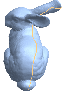
Now find and visualize the path:

HighlightMesh[mesh, Line@FindShortestPath[IGMeshGraph[mesh], 2920, 3115]]

Mathematica graphics

Mesure the path length:

GraphDistance[IGMeshGraph[mesh], 2920, 3115]
(* 0.250329 *)
$\endgroup$
9
$\begingroup$

Graph Based Algorithm (Dijkstra)

One algorithm that already gives an approximation to the shortest path (which approximates a geodesic), is the algorithm already implemented in Mathematica for testing shortest paths in graphs (FindShortestPath[] see Documentation or the implementation by Quantum Oli here). By treating the mesh as a graph one can get an estimate for the shortest path confined to go along edges. This is ok for an estimate, however gives something akin to a “triangular-Manhattan” distance on the mesh rather than the minimal distance and the geodesic. This can be implemented as follows:

a = BoundaryDiscretizeRegion[Ball[{0, 0, 0}, 1], 
   MaxCellMeasure -> {"Length" -> 1}, PrecisionGoal -> 3];
pts = MeshCoordinates[a];
edges = MeshCells[a, 1] /. Line[p_] :> p ;
tri = MeshCells[a, 2] /. Polygon[p_] :> p;
g = Graph[edges, GraphHighlight -> {1, 20}, 
   EdgeWeight -> PropertyValue[{a, 1}, MeshCellMeasure]];
path = PathGraph@FindShortestPath[g, 1, 20];
HighlightGraph[g, path]
Show[{a, Graphics3D[{Thick, Red, Line[pts[[VertexList[path]]]]}], 
  Graphics3D[{Black, Ball[pts[[{1, 20}]], 0.01]}]}, Axes -> True]

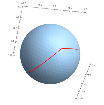
and gives as an example path:

Graph based "geodesic"

Note the kink in the path, hinting at the approximate nature of this algorithm.

$\endgroup$
5
  • 3
    $\begingroup$ I have used this extensively, but it is quite problematic, and depends significantly on the mesh structure. I am glad I found the diffusion based solution in this thread. $\endgroup$
    – Szabolcs
    Commented Mar 27, 2017 at 11:41
  • $\begingroup$ @Szabolcs. To be honest the solution to calculate shortest paths I used in the Geodesics in Heat Algorithm answer is also not that ideal and probably suffers from similar issues, even though it will pass through vertices in order of decreasing distance. Perhaps it could be worth using the vertex distances to guide the exact algorithm? $\endgroup$
    – Dunlop
    Commented Mar 27, 2017 at 17:58
  • $\begingroup$ Please consider putting this together as a function for the Wolfram Function Repository. $\endgroup$ Commented Apr 19, 2020 at 16:40
  • 1
    $\begingroup$ You can now shrink this code down somewhat with MeshConnectivityGraph which appeared in the 12.1 release in 2020. $\endgroup$
    – flinty
    Commented Nov 16, 2020 at 17:44
  • $\begingroup$ @flinty Feel free to edit or change this. I will need a bit of time before I get round to it. Thanks for the heads up though! $\endgroup$
    – Dunlop
    Commented Nov 16, 2020 at 18:22

Your Answer

By clicking “Post Your Answer”, you agree to our terms of service and acknowledge you have read our privacy policy.

Not the answer you're looking for? Browse other questions tagged or ask your own question.