46
$\begingroup$

I'm visualizing some hydrogen like atomic orbitals. For looking at plane slices of the probability density, the DensityPlot function works well, and with something like:

Manipulate[
 DensityPlot[ psi1XYsq[u, v, z], {u, -w, w}, {v, -w, w} ,
  Mesh -> False, Frame -> False, PlotPoints -> 45,
  ColorFunctionScaling -> True, ColorFunction -> "SunsetColors"]
 , {{w, 10}, 1, 20}
 , {z, 1, 20, 1}
 ]

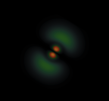
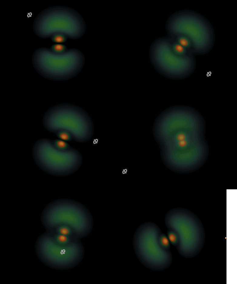
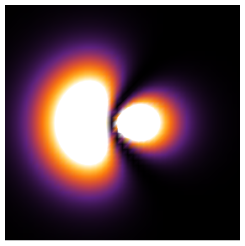
I can get a nice plot hybrid orbital sample plot in x y plane

I was hoping that there was something like a DensityPlot3D so that I could visualize these in 3D, but I don't see such a function. I was wondering how DensityPlot be simulated using other plot functions, so that the same idea could be applied to a 3D plot to construct a DensityPlot3D like function?

$\endgroup$
6
  • 4
    $\begingroup$ You may be interested in heatmap density 3D $\endgroup$
    – Kuba
    Commented Sep 15, 2013 at 16:33
  • 3
    $\begingroup$ Or how to visualize 4D function $\endgroup$
    – Kuba
    Commented Sep 15, 2013 at 16:34
  • 3
    $\begingroup$ Image3D works, apart from interpolation. A question arises, though: how you would be able to interpret the results? In general, isosurfaces are much more practical than images which look like fuzzy, vague clouds at best, opaque mass with hidden internal structure at worst. $\endgroup$
    – kirma
    Commented Sep 15, 2013 at 16:47
  • 5
    $\begingroup$ @kirma "fuzzy, vague clouds" - sounds like an orbital ;) $\endgroup$
    – Kuba
    Commented Sep 15, 2013 at 16:49
  • 3
    $\begingroup$ There is now DensityPlot3D in version 10.2. In the Applications section, there is an example of visualizing hydrogen orbitals. $\endgroup$ Commented Jul 9, 2015 at 15:56

4 Answers 4

29
$\begingroup$

In the version 10.2, there is a builtin DensityPlot3D function, which can be used to visualize orbitals.

a0=1;

ψ[{n_, l_, m_}, {r_, θ_, ϕ_}] :=With[{ρ = 2 r/(n a0)}, 
 Sqrt[(2/(n a0))^3 (n - l - 1)!/(2 n (n + l)!)] Exp[-ρ/2] ρ^
  l LaguerreL[n - l - 1, 2 l + 1, ρ] SphericalHarmonicY[l, 
   m, θ, ϕ]]

DensityPlot3D[(Abs@ψ[{3, 2, 0}, {Sqrt[x^2 + y^2 + z^2], 
     ArcTan[z, Sqrt[x^2 + y^2]], ArcTan[x, y]}])^2, {x, -10 a0, 
  10 a0}, {y, -10 a0, 10 a0}, {z, -15 a0, 15 a0}, 
 PlotLegends -> Automatic]

enter image description here

Or use ListDensityPlot3D:

data = Block[
 {nψ = 
   CompileWaveFunction[ψ[3, 1, 0, r, ϑ, φ]], data, vol},
 Table[Abs[nψ[x, y, z]]^2, {z, -20, 20, 0.25}, {y, -20, 20, 0.25}, {x, -20, 20, 0.25}]];

ListDensityPlot3D[data]

enter image description here

The function definition of the wave function is the same as in the other answer in this question.

$\endgroup$
8
  • $\begingroup$ I wonder how fast it is. Like Image3D? $\endgroup$
    – Jens
    Commented Jul 13, 2015 at 20:56
  • $\begingroup$ @Jens It seems to be slightly slower in giving back the result than Image3D on my computer. I just realized I'm using a library computer which is much powerful than my old laptop, so I compared the two again on the same machine I'm using, ListDensityPlot3D seem to slightly slower. $\endgroup$ Commented Jul 13, 2015 at 21:07
  • $\begingroup$ @RunnyKine Yes. It appeared in the user portal. Our university has a site license, and I received the email notice several days ago, but the new version only appeared today in my user portal. $\endgroup$ Commented Jul 13, 2015 at 21:19
  • 2
    $\begingroup$ @Jens I think the chief advantage of DensityPlot3D over Image3D is in OpacityFunction and OpacityFunctionScaling. Combined with ColorFunction, it really is a powerful tool for changing what is visible in the function. $\endgroup$
    – rcollyer
    Commented Jul 14, 2015 at 13:57
  • $\begingroup$ It's a bit slow on my computer, I guess ListDensityPlot3D is not well optimized. $\endgroup$
    – RandomEli
    Commented Jul 21, 2015 at 20:00
36
$\begingroup$

In an presentation by Markus van Almsick, he gives an solution to visualize atomic orbitals using Image3D.

Radius wave function (hydrogen):

R[n_Integer?Positive, l_Integer?NonNegative, r_] :=
 Block[{ρ = (2 r)/n}, 
   Sqrt[(2/n)^3 (n - l - 1)!/(2 n (n + l)!)] E^(-ρ/2) ρ^l LaguerreL[n - l - 1, 2 l + 1, ρ]] /; l < n

full wave function:

ψ[n_, l_, m_, r_, ϑ_, φ_] := ψ[n, l, m, r, ϑ, φ] = 
  FullSimplify[R[n, l, r] SphericalHarmonicY[l, m, ϑ, φ], {r >= 0, ϑ ∈ Reals, φ ∈ Reals}]


CompileWaveFunction = Compile[{{x, _Real}, {y, _Real}, {z, _Real}},
   Block[{ρ = x^2 + y^2, r, ϑ, φ},
    If[ρ > 0,
     r = Sqrt[ρ + z^2]; ϑ = ArcCos[z/r]; φ = ArcTan[x, y],
     r = Abs[z]; ϑ = π/2 Sign[z]; φ = 0];
     #
    ],
   CompilationTarget -> "C"
   ] &;

color function:

colorFunction = (Blend[{
      {0., RGBColor[0.7, 0.8, 1., 0.]}, 
      {0.1, RGBColor[0., 0.7, 0.1, 0.012]}, 
      {0.4, RGBColor[1., 0.1, 0.03169, 0.06723]}, 
      {1., RGBColor[1., 0.95051, 0., 0.10963]}}, #] &)

plot 3p orbital

Block[
 {nψ = 
   CompileWaveFunction[ψ[3, 1, 0, r, ϑ, φ]], data, vol},
 data = Table[Abs[nψ[x, y, z]]^2, {z, -20, 20, 0.25}, {y, -20, 20, 0.25}, {x, -20, 20, 0.25}];
 vol = RawArray["Byte", Round[(255/Max[data]) data]];
 Image3D[vol, "Byte", Background -> Black, 
  Method -> {"FastRendering" -> True, "InterpolateValues" -> True}, 
  ColorFunction -> colorFunction, BoxRatios -> 1]
 ]

enter image description here

it's quite smooth to rotate the Image3D object

enter image description here


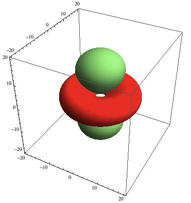
We can also visualize the atomic orbital by plotting the isosurface:

Block[{nψ = CompileWaveFunction[ψ[3, 2, 0, r, ϑ, φ]]},
 ContourPlot3D[Abs[nψ[x, y, z]]^2, {x, -20, 20}, {y, -20, 20}, {z, -20, 20}, 
  PlotPoints -> 15, Contours -> {0.00002}, 
  ColorFunction -> Function[{x, y, z}, ColorData["Rainbow"]@Rescale[Arg[nψ[x, y, z]], {-π, π}]], 
  ColorFunctionScaling -> False, Mesh -> None]
 ]

enter image description here

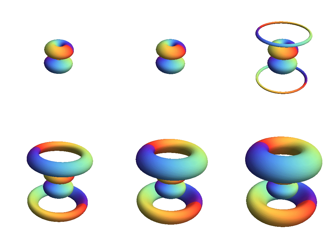
and make a animation showing different isosurfaces

plots = ParallelTable[
   Block[{nψ = CompileWaveFunction[ψ[4, 2, 1, r, ϑ, φ]]}, 
     ContourPlot3D[
      Abs[nψ[x, y, z]]^2, {x, -20, 20}, {y, -20, 20}, {z, -20, 20}, PlotPoints -> 17, Contours -> {ct}, 
      ColorFunction -> Function[{x, y, z}, ColorData["Rainbow"]@Rescale[Arg[nψ[x, y, z]], {-π, π}]], 
      Boxed -> False, Axes -> False, ColorFunctionScaling -> False, Mesh -> None, 
      ViewPoint -> {0.98, -2.76, 1.7}, ViewVertical -> {-0.004, -0.117, 0.993}]],
   {ct, 0.00003, 0.000015, -0.0000005}
   ];
ListAnimate[plots]

enter image description here

$\endgroup$
27
$\begingroup$

I recently revisited this, and found that RegionPlot3D is by far the fastest way to plot orbitals, compared to Image3D and ContourPlot3D. I was surprised by the difference, so I thought it's worth posting this.

In addition, I also made the process of choosing the plot parameters automatic, based on simple estimates for the size of the orbital wave function. So you don't have to find the right contour value by trial and error. This automation allows me to plot large numbers of orbitals in one go.

Below, I'm plotting the first ten orbitals in a systematic table, and the whole table takes about as long as doing one or two such plots using ContourPlot3D (depending on what functions I try). There was also no need to compile any of the functions, making the code quite straightforward.

Clear[rMin, rMax, r, θ, ϕ];
{rMin[n_, l_], rMax[n_, l_]} = 
  r /. Simplify[
    Solve[(l (l + 1))/r^2 - 2/r == -(1/n^2), r], 
    n > 0];

sphericalToCartesian = 
  Thread[{r, θ, ϕ} -> {Sqrt[x^2 + y^2 + z^2], 
     ArcCos[z/Sqrt[x^2 + y^2 + z^2]], Arg[x + I y]}];

ψ[n_, l_, m_][r_, θ_, ϕ_] := 
 Sqrt[ (n - l - 1)!/(n + l)!] E^(-(r/n)) ((2 r)/n)^l 2/
  n^2 LaguerreL[n - l - 1, 2 l + 1, (2 r)/n] SphericalHarmonicY[l, 
   m, θ, ϕ]

ClearAll[plotOrbital];
plotOrbital[f_, range_, contour_, opt : OptionsPattern[]] := 
 RegionPlot3D[
  Evaluate[Abs[f[r, θ, ϕ] /. sphericalToCartesian]^2 > 
    contour], {x, -range, range}, {y, -range, range}, {z, -range, 
   range}, opt, Mesh -> False, PlotPoints -> 35, PlotStyle -> Orange, 
  Lighting -> "Neutral", PlotTheme -> "Classic"]

grid = Table[
   Labeled[plotOrbital[ψ[n, l, m], 2 n^2, .05/n^6], 
    Row[{"n = ", n, ", ℓ = ", l, ", m = ", m}]], {n, 1, 
    3}, {l, 0, n - 1}, {m, 0, l}];

TableForm[grid]
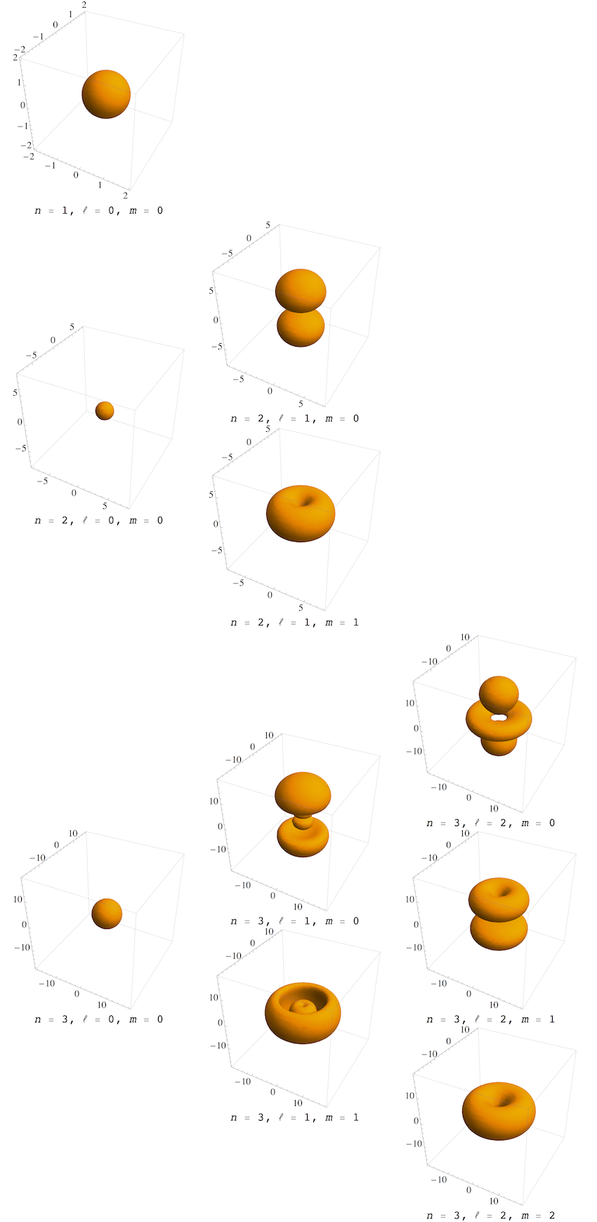
orbitals

Above, the complete hydrogenic orbital wave function is ψ. Given the principal quantum number n, the energy is known. Setting the energy equal to the effective potential yields the classical turning points, {rMin[n_, ℓ_], rMax[n_, ℓ_]}. This is used to determine the required plot size automatically: If the linear dimension r scales with $n^2$, then the volume scales with $n^6$. For a normalized wave function, we can then estimate that the probability density at a typical point will decrease with $1/n^6$. Therefore, I choose the threshold for the equi-probability contour to scale with this factor. Here is a check to verify what I said about the length scale:

Simplify[rMax[n, 0], n > 0]

(* ==> 2 n^2 *)

This is the largest achievable radius because I set the angular momentum l to zero.

In sphericalToCartesian, I write down how to convert to Cartesian coordinates (instead of using built-in functions which differ too much between Mathematica versions).

plotOrbital does the plotting for a given wave function f. In producing the grid of orbitals, I choose the parameters as described above.


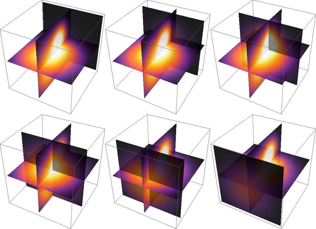
Edit: volumetric slices

To show that the RegionPlot approach is also able to provide multiple contours, and to show how these layered contours can give us information about the volume in 3D, here I first combine several outputs of plotOrbital with different contour values in a single Show. The surfaces have been given their own PlotStyle. Then I put the resulting 3D graphics in a Manipulate that allows you to slice through the layers in real time:

With[{n = 3, l = 2, m = 0}, 
 orb = Show[
   Table[plotOrbital[ψ[n, l, m], 2 n^2, c/n^6, 
     PlotStyle -> Directive[Opacity[0.6`], Hue[c]]], {c, 0.3`, 
     0.05`, -0.04`}], PlotRange -> All, BoxRatios -> Automatic]]

With[{n = 3},
 Manipulate[
  Show[orb, Boxed -> False, Axes -> False, 
   ViewVector -> {{35, -35, 5}, {0, 0, 0}}, ViewAngle -> Pi/4, 
   PlotRange -> {{-#, #}, {y, #}, {-#, #}} &[2 n^2]], {y, -2 n^2, 
   2 n^2}]]

slices

The trick to get slices and hollow spaces between layers in RegionPlot3D is to cut off the plot with a reduced PlotRange. To still keep the object fixed in the view port (instead of moving around to stay centered with the changing PlotRange), I add fixed values for the ViewVector and ViewAngle. This trick using PlotRange doesn't work if you cut the range off directly inside the RegionPlot3D. You have to do it after the fact with Show.

Again, the drawing of multiple layers is very fast using RegionPlot3D. It could even be sped up more using ParallelTable.

Edit2

In Mathematica version 10, the volumetric slices can also be achieved using the ClipPlanes option:

With[{n = 3}, 
 Manipulate[
  Show[orb, Boxed -> False, Axes -> False, 
   ViewVector -> {{35, -35, 5}, {0, 0, 0}}, ViewAngle -> Pi/4, 
   ClipPlanes -> {{0, 1, 0, 1.2 y}}], {{y, 0}, -n^2, n^2}]]

The output is the same as in the previous animation.
$\endgroup$
1
  • 1
    $\begingroup$ That's fantastic! Indeed RegionPlot3D is much faster. And it also solves the problem of holes in ContourPlot3D. $\endgroup$ Commented Feb 21, 2015 at 22:27
24
$\begingroup$

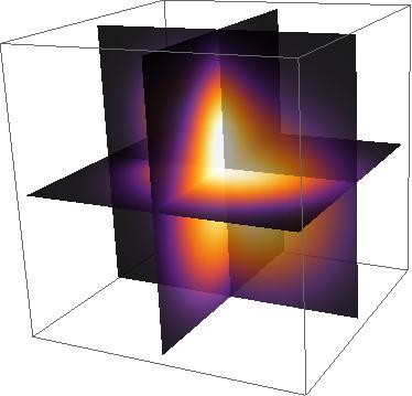
My preferred method for this kind of thing is projecting each dimension onto a plane and then combining them together. I think MATLAB has similar functionality. Mind you, the answers and comments on my question about projecting are right in pointing out that this will become inefficient for high polygon counts (essentially more PlotPoints) so if you want to Manipulate in a smooth way, you may want to use Texture. See this relevant question for details on that.

Now, I haven't got your function psi1XYsq so I will pick a double gaussian:

E^(-(x^2 + (y - 2)^2 + (z - 3)^2)/10) + E^(-((x + 1)^2 + (y + 2)^2 + (z + 2)^2)/25)

The idea is to use something similar to the function @Jens is using in his answer to How to make a drop-shadow for a Graphics3D objects?.

Block[{d1, d2, d3, function, options, opacity, x0, y0, z0, min, max},
 {min, max} = {-9, 9};
 {x0, y0, z0} = {0., 0., 0.};
 opacity = 0.9;
 function[x_, y_, z_] := 
  E^(-(x^2 + (y - 2)^2 + (z - 3)^2)/10) + 
   E^(-((x + 1)^2 + (y + 2)^2 + (z + 2)^2)/25);
 options = Sequence @@ {PlotPoints -> 45, Mesh -> None, 
    ColorFunctionScaling -> False, ColorFunction -> "SunsetColors"};
 d1 = First@DensityPlot[function[x, y, z0], {x, min, max}, {y, min, max}, 
     Evaluate@options] /. {x_?AtomQ, y_?AtomQ} -> {x, y, z0};
 d2 = First@DensityPlot[function[x, y0, z], {x, min, max}, {z, min, max}, 
     Evaluate@options] /. {x_?AtomQ, z_?AtomQ} -> {x, y0, z};
 d3 = First@DensityPlot[function[x0, y, z], {y, min, max}, {z, min, max}, 
     Evaluate@options] /. {y_?AtomQ, z_?AtomQ} -> {x0, y, z};
 Show[Graphics3D[{d1, d2, d3}, Lighting -> "Neutral"] /. 
   GraphicsComplex[xx__] -> {Opacity[opacity], GraphicsComplex[xx]}]
 ]

3d image

The code is straightforward: min, max define the range for each variable, {x0, y0, z0} define the projection planes, and opacity the Opacity. You will notice I have turned off ColorFunctionScaling so that each slice is bright according to an absolute value and they merge together nicely. If your function is not normalised you may want to normalise it before doing that.

If you can afford lowering the PlotPoints, Manipulate isn't too bad, and you can make animations that look like volumetric rendering (apologies for the 300K gif):

Table[Block[{d1, d2, d3, function, options, opacity, x0, y0, z0, min, 
    max},
   {min, max} = {-9, 9};
   {x0, y0, z0} = {0., t, 0.};
   opacity = 0.9;
   function[x_, y_, z_] := 
    E^(-(x^2 + (y - 2)^2 + (z - 3)^2)/10) + 
     E^(-((x + 1)^2 + (y + 2)^2 + (z + 2)^2)/45);
   options = 
    Sequence @@ {PlotPoints -> 25, Mesh -> None, 
      ColorFunctionScaling -> False, 
      ColorFunction -> "SunsetColors"};
   d1 = First@
      DensityPlot[function[x, y, z0], {x, min, max}, {y, min, max}, 
       Evaluate@options] /. {x_?AtomQ, y_?AtomQ} -> {x, y, z0};
   d2 = First@
      DensityPlot[function[x, y0, z], {x, min, max}, {z, min, max}, 
       Evaluate@options] /. {x_?AtomQ, z_?AtomQ} -> {x, y0, z};
   d3 = First@
      DensityPlot[function[x0, y, z], {y, min, max}, {z, min, max}, 
       Evaluate@options] /. {y_?AtomQ, z_?AtomQ} -> {x0, y, z};
   Show[Graphics3D[{d1, d2, d3}, Lighting -> "Neutral"] /. 
     GraphicsComplex[xx__] -> {Opacity[opacity], 
       GraphicsComplex[xx]}]
   ], {t, 9, -9, -1.5}];
Export["3d.gif", %];

3dGif

$\endgroup$
3
  • $\begingroup$ What does your {x_?AtomQ, y_?AtomQ} -> {x, y, z0} replacement in this code do? $\endgroup$ Commented Sep 17, 2013 at 22:17
  • $\begingroup$ I adds a third dimension to every pair of 2d coordinates of the density plot. $\endgroup$
    – gpap
    Commented Sep 17, 2013 at 23:46
  • 1
    $\begingroup$ The new (in 10.4) function SliceDensityPlot3D automates this. $\endgroup$
    – rcollyer
    Commented May 19, 2016 at 15:13

Your Answer

By clicking “Post Your Answer”, you agree to our terms of service and acknowledge you have read our privacy policy.

Not the answer you're looking for? Browse other questions tagged or ask your own question.