Precompiling a Whittaker function

Question

Is there a way to speed up the evaluation of special functions in Mathematica? I am particularly interested in the Whittaker W function. For instance, the following piece of code:

f[x_, y_] := Re[WhittakerW[2, I*x, y]];
RepeatedTiming[f[0.4, 2]]

takes about the same amount of time to execute as does the following one

g = Compile[{{x, _Real}, {y, _Real}}, Re[WhittakerW[2, I*x, y]]];
RepeatedTiming[g[0.4, 2]]

I was hoping that by precompiling the function I would sacrifice the versatility but gain performance. Yet although the versatility did get lost, the performance didn't change one bit. Any suggestions?

Answer 1

Original answer

J.M.'s answer in About multi-root search in Mathematica for transcendental equations shows how to approximate an analytic function in a finite interval by its Chebyshev series. We can do the same here, if we avoid the singularity at zero.

Here is a utility function for evaluating a Chebyshev expansion whose coefficients are stored in the array c. We can even compile it, using the identity $T_n(x) = \cos(n\,\arccos x)$. [Edit notice: See improvements to chebeval below.]

Clear[chebeval];
chebeval[c_] :=
  Compile[{x}, c.Table[Cos[(n - 1) ArcCos[x]], {n, Length@c}]];
chebeval[c_, x_?NumericQ] :=
 c.Table[ChebyshevT[n - 1, x], {n, Length@c}]

Example. We'll fix x = 0.4 and approximate over 1 <= y <= 4.

w = WhittakerW[2, I*0.4, #] &;
{ymin, ymax} = {1, 4};
n = 32;
cnodes = Rescale[N[Cos[Pi Range[0, n]/n], 20], {-1, 1}, {ymin, ymax}];
wcoeff = Sqrt[2/n] FourierDCT[w /@ cnodes, 1];
wcoeff[[{1, -1}]] /= 2;
Clear[wcheb];
wcheb[y_] := chebeval[wcoeff, Rescale[y, {ymin, ymax}, {-1, 1}]];
wcomp = With[{w = chebeval[wcoeff]}, w[Rescale[#, {ymin, ymax}, {-1, 1}]] &];

It's accurate to almost machine precision:

Plot[
 (Re[w[y]] - Re@wcheb[y]) / ($MachineEpsilon + $MachineEpsilon Abs@Re[w[y]]),
 {y, ymin, ymax}]

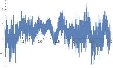
Error relative to precision and accuracy goals of $MachineEpsilon.

The compiled version is especially faster:

Re@w[2] // RepeatedTiming
Re@wcheb[2] // RepeatedTiming
Re@wcomp[2] // RepeatedTiming
(*
  {0.0011, -0.129877}
  {0.00017, -0.129877}
  {9.03*10^-6, -0.129877}
*)

Greater speed and greater accuracy

J.M points out that Clenshaw's algorithm for computing truncated Chebyshev series is numerically more stable, and "algorithmically faster," if that is the right way to say it. I mean that in terms of floating-point operations, it should be faster than computing trigonometric functions. However internal optimization Cos and ArcCos may mean it is computed faster than compiled Mathematica code. This is the case on my Mac and the Cos/ArcCos implementation of chebeval. If you can compile to C, then the Clenshaw method will probably be faster; it is on my machine. Then Clenshaw algorithm has about 70% of the error of the Cos/ArcCos implementation on average.

Here are three routines for computing a truncated Chebyshev series. One is a more efficient "vectorized" variation on the Cos/ArcCos method above. The other two implement Clenshaw's algorithm, the only difference between them is that one is compiled to C. Further notes on speed and accuracy are given further down.

Clear[chebeval];
chebeval["TrigVectorized"][c_?VectorQ] := With[{deg = Length@c - 1},
   Compile[{x}, Block[{ac = ArcCos[x]}, c.Cos[Range[0, deg] ac]],
    RuntimeAttributes -> {Listable}]
   ];
chebeval["Clenshaw"][c0 : {__Real}] :=
  With[{c1 = Reverse[c0], deg = Length@c0 - 1},
   Compile[{x},
    Block[{c = c1, s = 0., s1 = 0., s2 = 0.},
     Do[
      s = c[[i]] + 2 x*s1 - s2;
      s2 = s1; s1 = s,
      {i, deg}];
     Last@c + x*s1 - s2
     ],
    RuntimeAttributes -> {Listable}]
   ];
chebeval["Clenshaw-C"][c0 : {__Real}] :=
  With[{c1 = Reverse[c0], deg = Length@c0 - 1},
   Compile[{x},
    Block[{c = c1, s = 0., s1 = 0., s2 = 0.},
     Do[
      s = c[[i]] + 2 x*s1 - s2;
      s2 = s1; s1 = s,
      {i, deg}];
     Last@c + x*s1 - s2
     ],
    RuntimeAttributes -> {Listable}, Parallelization -> True,
    CompilationTarget -> "C"]
   ];

Note that if complex values are needed, then the local variables in the Clenshaw routines should be initialized to complex values, that is, s = 0. + 0. I, s1 = 0. + 0. I, s2 = 0. + 0. I; and of course, the argument pattern c0 : {__Real} would need to be changed to something like c0_?VectorQ. (See also the notes on speed below.)

Timings

y0 = RandomReal[{ymin, ymax}, 10^5];

Needs["GeneralUtilities`"];
TableForm@Join[
 {{"Name", 1, Length[y0]}},
 Table[
  wcomp = chebeval[s][Re@wcoeff];
  {s, AccurateTiming@Re@wcomp[Rescale[2, {ymin, ymax}, {-1, 1}]],
   AccurateTiming@Re@wcomp[Rescale[y0, {ymin, ymax}, {-1, 1}]]},
  {s, {"Clenshaw", "TrigVectorized", "Clenshaw-C"}}]
 ]

Each is faster than the timing 9.03*10^-6 of the original answer (on a single element).

Accuracy

There is no difference between the two Clenshaw routines. They are somewhat better than the Cos/ArcCos method.

  (* input and values *)
input = Range[N@ymin, N@ymax, (ymax - ymin)/10013.];
wvec = w[input];
input = Rescale[input, {ymin, ymax}, {-1, 1}];
trig = chebeval["TrigVectorized"][Re@wcoeff][input];
clen = chebeval["Clenshaw-C"][Re@wcoeff][input];
  (* norms -- see notes below *)
svn2 = NDSolve`ScaledVectorNorm[2, {$MachineEpsilon, $MachineEpsilon/8}];
svnInf1 = NDSolve`ScaledVectorNorm[Infinity, {$MachineEpsilon, $MachineEpsilon}];
svnInf8 = NDSolve`ScaledVectorNorm[Infinity, {$MachineEpsilon, $MachineEpsilon/8}];

Grid[
 {{"Norm"[p, a], "Cos/ArcCos", "Clenshaw"},
  {"RMS"[ϵ, ϵ/8], svn2[trig - wvec, wvec], svn2[clen - wvec, wvec]},
  {∞[ϵ, ϵ], svnInf1[trig - wvec, wvec], svnInf1[clen - wvec, wvec]},
  {∞[ϵ, ϵ/8], svnInf8[trig - wvec, wvec], svnInf8[clen - wvec, wvec]}},
 Dividers -> {{False, True}, {False, True}}
 ]

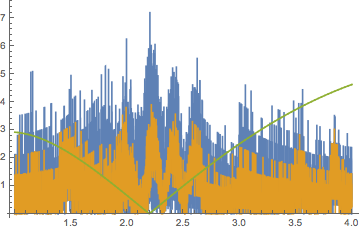
Below is a pointwise comparision of the Cos/ArcCos and Clenshaw methods. Note that as w[y] approaches zero (the green line shows 5 * w[y]), the scaled error increases; this depends on the "accuracy" parameter $MachineEpsilon/8

ListLinePlot[
 {MapThread[svnInf8[{#1 - #2}, {#2}] &, {trig, wvec}],
  MapThread[svnInf8[{#1 - #2}, {#2}] &, {clen, wvec}],
  Abs[5 wvec]},
 DataRange -> {ymin, ymax}, PlotRange -> All
 ]

The W function (green); scaled error, Clenshaw (yellow); scaled error, Cos/ArcCos (blue)

Some notes on speed

• In this case the function is real-valued, but FourierDCT returns coefficients with negligible imaginary parts. It's faster to compute with real than with complex numbers, so getting rid of the imaginary parts with Re@wcoeff helps slightly with speed, especially with the slower (WVM) Clenshaw routine. Of course, one can work with complex coefficients as indicated above.
• The usual description of the Clenshaw algorithm counts down from the $n^{\rm th}$ coefficient to the zeroth. However in the compiler, Do[.., {i, max, min, -1}] is slower than Do[.., {i, min, max}]. Hence, we reverse the coefficient array before compiling (a one-time cost).
• The relative timings may vary. It seems likely that the MKL would use the built-in hardware arc cosine command on my Intel i7 chip and that Mathematica would use the MKL for machine-precision computation. This may explain why the WVM-compiled Cos/ArcCos routine is faster than the WMV-compiled Clenshaw routine, and why compiling to C reverses the comparison. (Compiling the Cos/ArcCos routine to C makes no difference in speed since it is a one-liner with no loops.)

Some notes on precision and accuracy

• The typical measure of function approximation in Mathematica is the "scaled vector norm," described in the tutorial Norms in NDSolve. A given PrecisionGoal of $pg$ and AccuracyGoal of $ag$ corresponds to tolerances $t_p=10^{-pg}$ and $t_a=10^{-ag}$. An absolute error $\delta$ related to an exact value $v$ has the scaled error of $$se = {\delta \over t_a + t_p\,|v|}$$ The joint precision/accuracy goal is considered to be "met" if $se < 1$. Just what this means changes depending on the relative sizes of $t_a$ and $t_p\,|v|$. When $t_a$ is much greater (so that $|v|$ is very small), the goal is met when the approximation accurate to $-\log_{10}(t_a)$ decimal places; that is, it depends on the absolute error. At the other extreme, the goal is met with the first $-\log_{10}(t_p)$ digits are accurate; that is, it depends on the relative error.
• svn = NDSolve`ScaledVectorNorm[p, {precTol, accTol}] returns a function svn that svn[eVec, vVec] computes the $p$-norm of a vector of absolute errors eVec scaled relative to a vector of exact values vVec with the precision and accuracy tolerances precTol and accTol respectively. (See the linked tutorial on norms.)