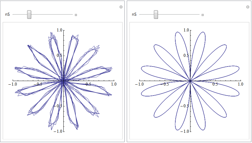
Mr. Wizard's answer indeed solves the problem of the ugly display. What's left to add is perhaps the more general question of why this seemingly trivial drawing problem is so slow in the first place.
The whole point of a Manipulate slider is, after all, that you want to see immediate effects in real time. And the difference to ListAnimate is that you want the real-time response to be a computed result, not in general a pre-rendered frame (because then we wouldn't need Manipulate in the first place).
So one should investigate the factors that slow down the displayed object in your manipulate. In this case, it has to do with the fact that ParametricPlot and other plotting functions try to choose a clever set of plot points and then do an interpolation to draw a smooth line. But trying to be clever can cost you time.
So if you want to run your Manipulate on a slow computer and still want high quality, that will mean the response to the slider action will become very sluggish. The output will look nice at all times, but the user experience will be bad. So you're between a rock and a hard place, unless you get rid of the time consuming step in the plot, i.e., the refinement and interpolation.
The solution then boils down to replacing ParametricPlot by ListParametricPlot (with lowest InterpolationOrder -> 1 which is the default). This is actually what I do quite often with DensityPlots, too (replace by ListDensityPlot or even ArrayPlot or Image). It's usually faster.
Here is what that would look like in the above example (keeping the over-wrapped angle variable just for consistency with the original):
Manipulate[
 ListPolarPlot[
  Table[{t, Sin[nS*t]}, {t, -5 Pi, 5 Pi, Pi/(20 + 15 nS)}],
  Joined -> True, InterpolationOrder -> 1], {nS, 1, 20, 1}]
You can leave out InterpolationOrder -> 1, but I put it in so you can compare what happens if it's replaced by InterpolationOrder -> 2.
In choosing the number of points to generate in the Table, I used the number of expected lobes as a parameter (the higher nS, the more detail we need). For this example, this doesn't give any speed advantage really, but I think it's worth keeping in mind when your functions get more complicated. The explicit choice of plot points in this list plot is essentially part of the user-interface design, in that you decide how much lag you like to accept for an increase in quality.
Edit
Here is an example of a polar plot where Manipulate becomes really painful - using PolarPlot but with a different function than given in the question. It's plotting the result of a numerical integration in "real time":
Manipulate[
 PolarPlot[NIntegrate[LaguerreL[nS, x], {x, 0, t}], {t, 0, 2 Pi},
  PlotPoints -> ControlActive[10, 60]], {nS, 1, 20, 1}]
Trying this on my machine, I can (with some patience) drag the slider to the max, but then have to wait quite some time for the final interpolated curve to appear. Then I try to drag the slider back to the left, and Mathematica becomes unresponsive for several seconds, not even drawing the ControlActive version of the plot. The CPU usage sticks at 100%. And this despite the fact that I limited even the high-quality number of plot points to 60.
Now delete the manipulate generated above and try the next one:
Manipulate[
 ListPolarPlot[
  Table[NIntegrate[LaguerreL[nS, x], {x, 0, t}], {t, 0,
    2 Pi, Pi/30}], Joined -> True], {nS, 1, 20, 1}]
Again it takes just as much patience to drag the slider all the way to the right. The difference here is that I have used ListPolarPlot and therefore was able to forego any attempts at interpolation. This means that the plot looks more angular than in the previous example, even though the number of plot points is the same as above.
But at least the Manipulate now responds much faster when I try to drag the slider back down. I'm pushing the performance limits here, so one should add a disclaimer: save your work before trying this.
The point here is: Manipulate seems to be utterly useless for this admittedly contrived example unless we can turn off interpolation. To do so, I used the ListPolarPlot version because by default it does not attempt interpolation. This means the final curves won't look entirely smooth, but (a) they look the same while dragging as they do when finished, and (b) the interface doesn't go into a coma.
There may be ways of getting ListPlot to perform a better here, but as far as I know, ListPolarPlot is the most straightforward way to get the control I need here.
Edit 2
Another good way to speed up the PolarPlot without using ListPolarPlot is to add MaxRecursion -> 0. This suppresses the iterative refinement of the point set on which the function is evaluated - and the advantage is that you can combine it more easily with Mr. Wizard's other suggestions.
Here are two closely related links that use both the List...Plot approach and the MaxRecursion approach. Either one can be superior, depending on the situation:


Manipulate[PolarPlot[Sin[nS*t], {t, -Pi, Pi}], {nS, 1, 20, 1}]is much better $\endgroup$