Solving $L=\frac{3}{2} \sqrt{4 \pi ^2 A^2+W^2}-\frac{\sqrt{5 W \sqrt{4 \pi ^2 A^2+W^2}+6 \pi ^2 A^2+3 W^2}}{\sqrt{2}}+\frac{3 W}{2}$ for $W$

Question

When I solve the aforementioned equation for $W$ or $A$ on Mathematica I get a long and ugly equation in return, namely one of the solutions for $W$ is: (attempt to read at your own health)

Solve[L == (3 W)/2 + (3 Sqrt[4 A^2 Pi^2 + W^2])/2 - Sqrt[6 A^2 Pi^2 + 3 W^2 +
  5 W Sqrt[4 A^2 Pi^2 + W^2]]/Sqrt[2], W]

$W=\frac{3 L}{10}-\frac{1}{2} \sqrt{\frac{\sqrt[3]{-243200 \pi ^6 A^6+176832 L^2 \pi ^4 A^4+3600 L^4 \pi ^2 A^2+2160 L^6+\sqrt{-7962624000 \pi ^{12} A^{12}-8626176000 L^2 \pi ^{10} A^{10}+717410304 L^4 \pi ^8 A^8+3308138496 L^6 \pi ^6 A^6+911879424 L^8 \pi ^4 A^4+17252352 L^{10} \pi ^2 A^2+4672512 L^{12}}}}{15 \sqrt[3]{2}}+\frac{9 L^2}{25}-\frac{4}{15} \left(10 \pi ^2 A^2+3 L^2\right)+\frac{4 \sqrt[3]{2} \left(640 \pi ^4 A^4-246 L^2 \pi ^2 A^2-3 L^4\right)}{15 \sqrt[3]{-243200 \pi ^6 A^6+176832 L^2 \pi ^4 A^4+3600 L^4 \pi ^2 A^2+2160 L^6+\sqrt{-7962624000 \pi ^{12} A^{12}-8626176000 L^2 \pi ^{10} A^{10}+717410304 L^4 \pi ^8 A^8+3308138496 L^6 \pi ^6 A^6+911879424 L^8 \pi ^4 A^4+17252352 L^{10} \pi ^2 A^2+4672512 L^{12}}}}}-\frac{1}{2} \sqrt{-\frac{\sqrt[3]{-243200 \pi ^6 A^6+176832 L^2 \pi ^4 A^4+3600 L^4 \pi ^2 A^2+2160 L^6+\sqrt{-7962624000 \pi ^{12} A^{12}-8626176000 L^2 \pi ^{10} A^{10}+717410304 L^4 \pi ^8 A^8+3308138496 L^6 \pi ^6 A^6+911879424 L^8 \pi ^4 A^4+17252352 L^{10} \pi ^2 A^2+4672512 L^{12}}}}{15 \sqrt[3]{2}}+\frac{18 L^2}{25}-\frac{8}{15} \left(10 \pi ^2 A^2+3 L^2\right)-\frac{4 \sqrt[3]{2} \left(640 \pi ^4 A^4-246 L^2 \pi ^2 A^2-3 L^4\right)}{15 \sqrt[3]{-243200 \pi ^6 A^6+176832 L^2 \pi ^4 A^4+3600 L^4 \pi ^2 A^2+2160 L^6+\sqrt{-7962624000 \pi ^{12} A^{12}-8626176000 L^2 \pi ^{10} A^{10}+717410304 L^4 \pi ^8 A^8+3308138496 L^6 \pi ^6 A^6+911879424 L^8 \pi ^4 A^4+17252352 L^{10} \pi ^2 A^2+4672512 L^{12}}}}-\frac{\frac{216 L^3}{125}-\frac{48}{25} \left(10 \pi ^2 A^2+3 L^2\right) L+\frac{48}{5} \left(L^2-2 A^2 \pi ^2\right) L}{4 \sqrt{\frac{\sqrt[3]{-243200 \pi ^6 A^6+176832 L^2 \pi ^4 A^4+3600 L^4 \pi ^2 A^2+2160 L^6+\sqrt{-7962624000 \pi ^{12} A^{12}-8626176000 L^2 \pi ^{10} A^{10}+717410304 L^4 \pi ^8 A^8+3308138496 L^6 \pi ^6 A^6+911879424 L^8 \pi ^4 A^4+17252352 L^{10} \pi ^2 A^2+4672512 L^{12}}}}{15 \sqrt[3]{2}}+\frac{9 L^2}{25}-\frac{4}{15} \left(10 \pi ^2 A^2+3 L^2\right)+\frac{4 \sqrt[3]{2} \left(640 \pi ^4 A^4-246 L^2 \pi ^2 A^2-3 L^4\right)}{15 \sqrt[3]{-243200 \pi ^6 A^6+176832 L^2 \pi ^4 A^4+3600 L^4 \pi ^2 A^2+2160 L^6+\sqrt{-7962624000 \pi ^{12} A^{12}-8626176000 L^2 \pi ^{10} A^{10}+717410304 L^4 \pi ^8 A^8+3308138496 L^6 \pi ^6 A^6+911879424 L^8 \pi ^4 A^4+17252352 L^{10} \pi ^2 A^2+4672512 L^{12}}}}}}}$

The above just makes the point that the solution can't be written by hand (or by mine at least).

So my question is, can I represent the solution using an easily-written function of $A$ and $L$ (for instance, as a infinite summation)?

Answer 1

It seems me that the answers of mathe and Yves Klett do not meet expectations of the author. The latter is as much as I have got it, to have a short analytical expression for the solution. Probably the author has an intention to use the result further in some analytical calculations, or to do something comparable. Am I right?

If yes, one should first of all be clear that what is already found is the exact solution, which is what it is. If you need the exact solution, you can only try to somewhat simplify it, as Yves Klett did, and after the simplification is done, that's it.

Another story, if you agree to have an approximate solution, which is expressed by a simple analytical formula. In that case I can contribute as follows. Here is your equation:

eq1 = L == (3 W)/2 + (3 Sqrt[4 A^2 Pi^2 + W^2])/2 -Sqrt[6 A^2
Pi^2 + 3 W^2 + 5 W Sqrt[4 A^2 Pi^2 + W^2]]/Sqrt[2]

First let us simplify a bit your equation by changing variables:

 eq2 = Simplify[
  eq1 /. {W -> 2 \[Pi]*A*x, L -> 2 \[Pi]*A*u}, {x > 0, A > 0}]

(*   3 (x + Sqrt[1 + x^2]) == 2 u + Sqrt[3 + 6 x^2 + 10 x Sqrt[1 + x^2]]   *)

Now let us consider the variable xas a new unknown and u as a parameter and solve with respect to x.

slX = Solve[eq2, x];

Its solutions are still too cumbersome. For this reason I do not give them below. One can make sure that there are four of them:

 slX // Length

(*  4  *)

And visualize them

    Plot[{slX[[1, 1, 2]], slX[[2, 1, 2]], slX[[3, 1, 2]], 
  slX[[4, 1, 2]]}, {u, 0, 4}, PlotStyle -> {Red, Blue, Green, Brown}]

giving the following:

Now one can approximate any of these solutions by some simple function. I will give the example with the first solution. First let us make a list out of it:

    lst = Select[Table[{u, slX[[1, 1, 2]]}, {u, 0.6, 1, 0.003}], 
   Im[#[[2]]] == 0 &];

Second, let us approximate it by a simple model:

model = a + b/(c + u);
ff = FindFit[lst, model, {a, b, {c, -0.63}}, u]
Show[{
  ListPlot[lst, Frame -> True, 
   FrameLabel -> {Style["u", 16, Italic], Style["x", 16, Italic]}],
  Plot[model /. ff, {u, 0.63, 1}, PlotStyle -> Red]
    }]

The outcome is the values of the model parameters:

(*    {a -> -0.418378, b -> 0.0290875, c -> -0.549429}   *)

and the plot enabling one to visually estimate the quality of the approximation:

Here the blue points come from the list, and the solid red line - from the approximation. Have fun!

Answer 2

I've fiddled with this on and off for a while now, hesitating to decide whether it was worth posting since another answer has already been accepted. The undocumented function, Experimental`OptimizeExpression, can be used to break down the solutions algebraically into common subexpressions, and it seemed like an approach worth sharing. On the other hand, this equation is essentially equivalent to a quartic polynomial:

Quit[]

eqn = L == (3 W)/2 + (3 Sqrt[4 A^2 Pi^2 + W^2])/2 - 
    Sqrt[6 A^2 Pi^2 + 3 W^2 + 5 W Sqrt[4 A^2 Pi^2 + W^2]]/Sqrt[2];
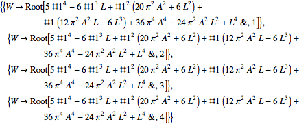
sols = W /. Solve[eqn, W];
poly = Collect[5 Times @@ (W - sols) // Expand // Simplify, W]
(*
  L^4 - 24 A^2 L^2 π^2 + 36 A^4 π^4 + (-6 L^3 + 12 A^2 L π^2) W +
   (6 L^2 + 20 A^2 π^2) W^2 - 6 L W^3 + 5 W^4
*)

The solutions turn out to resemble the standard quartic formula. Indeed, it might be just as easy to build up the solutions from the formula by hand from the polynomial derived below (perhaps using Mathematica to keep track of the algebraic steps). The expression will still be rather complicated due to the nature of the quartic formula and the coefficients, even if they appear to have some symmetry.

Different purposes might be fulfilled by being able to write expressions for the roots. Presumably the general goal would be to illuminate elements of the problem, but all we are given is an algebraic equation. In some cases an analytic approach might be more appropriate than an algebraic approach, or vice versa.

###Auxiliary functions###

Set up the equation and solutions; the solutions may be used to construct a polynomial with the same roots (the coefficient 5 is discovered by inspection).

The function Experimental`OptimizeExpression returns an expression of the form

Experimental`OptimizedExpression[Block[{vars}, var1 = val1; <>; varn = valn; expr]]

The variables have the form Compile`$nnn, where nnn represents a serial number, and represent subexpressions; if a subexpression appears more than once, it will be represented by the same variable. Unfortunately, the serial number increases throughout a session and the starting number depends on what evaluations have been done. (Execute Quit[] above to get the same numbering -- unless the numbering is version/system dependent.) The expression expr represents the optimized expression in terms of the variables. Preceding it, the variables are initialized. From this we can construct auxiliary functions for exploring the expression.

Experimental`OptimizeExpression takes an OptimizationLevel option and may be set to 0, 1, or 2. Subexpressions are stored in the returned Experimental`OptimizeExpression in a held Block in the form Compile`$nnn = expr. We can turn these Set expressions into Rule expressions that can be used to expand a given subexpression in terms of the next level of subexpressions. One can also replace the last expression inside Block with an arbitrary expression in terms of Compile`$nnn variable and it will be evaluated in terms of the subexpressions of the optimized expression.

optexpr = Experimental`OptimizeExpression[sols, OptimizationLevel -> 2];

(* get the initialization in terms of Rule *)
optrules = Most[(optexpr /. {Set -> Rule, CompoundExpression -> List})[[1, 2]]];

(* convert between Compile`$nnn symbol and the number nnn *)
compileSym = ToExpression["Compile`$" <> ToString[#]] &;
compileSymNo = ToExpression@StringDrop[SymbolName[#], 1] &;

(* get the range of the serial numbers of the variables *)
{minCompileNumber, 
   maxCompileNumber} = 
  Through[{Min, Max}[
    Cases[optexpr, 
     x_Symbol /; Context[x] === "Compile`" :> compileSymNo[x](*ToExpression@
     StringDrop[SymbolName[x],1]*), Infinity]]];

(* evaluate an expression in terms of Compile`$nnn variables *)
evalCompileExpr = ReplacePart[Function @@ optexpr, {1, -1, -1} :> Slot[1]];

The following shows the structure of the four roots determined by Experimental`OptimizeExpression. It reveals the typical structure of the roots of a quartic equation.

optoutput = optexpr[[1, -1, -1]]
(*
{Compile`$1 + Compile`$57 - Compile`$71/2, 
 Compile`$1 + Compile`$57 + Compile`$71/2, 
 Compile`$1 + Compile`$76 - Compile`$79/2, 
 Compile`$1 + Compile`$76 + Compile`$79/2}
*)

###Using the functions###

Executing expr /. optrules will expand the variables one step. What steps to take requires some judgment. If we expand optoutput, we see the structure of the quartic formula begin to unfold.

optoutput /. optrules
(*
{(3 L)/10 - Compile`$56/2 - Sqrt[Compile`$70]/2, (3 L)/10 - Compile`$56/2 + 
  Sqrt[Compile`$70]/2, (3 L)/10 + Compile`$56/2 - Sqrt[Compile`$78]/2, (3 L)/
  10 + Compile`$56/2 + Sqrt[Compile`$78]/2}
*)

{Compile`$70, Compile`$78} /. optrules
(*
{Compile`$58 + Compile`$59 + Compile`$60 + Compile`$61 + Compile`$69, 
 Compile`$58 + Compile`$59 + Compile`$60 + Compile`$61 + Compile`$77}
*)

{Compile`$69, Compile`$77} /. optrules
(*
{-((Compile`$67 Compile`$68)/4), (Compile`$67 Compile`$68)/4}
*)

The above calculations show we can write the solutions in the form

W -> 3 L / 10 ± d1 ± Sqrt[d2 ± d3] / 2

where

d1 = Compile`$56 / 2
d2 = Compile`$58 + Compile`$59 + Compile`$60 + Compile`$61
d3 = (Compile`$67 Compile`$68) / 4

and the first and third ± signs agree.

One can examine the actual expressions with evalCompileExpr, but, as I said, without the context of the problem, it's hard to see anything important lurking in the expressions.

We can break down the solution into bit-size pieces -- well, whiteboard-size pieces. One can see there is a large cube root that is repeated and larger square root. We can get them and replace with them with new variables Q and R as follows:

rootTerms = {Compile`$56/2, 
   Compile`$58 + Compile`$59 + Compile`$60 + Compile`$61, (Compile`$67 Compile`$68)/4};

simpRT = Simplify /@ evalCompileExpr[rootTerms];
q = First@Cases[simpRT, Power[Except[_?NumberQ], 1/3], Infinity];
Q -> q
cbrt = {q -> Q, 1/q -> 1/Q};
r = First@Cases[simpRT /. cbrt, Power[Except[_?NumberQ], 1/2], Infinity];
R -> r
sqrt = {r -> R, 1/r -> 1/R};
Thread[{d1, d2, d3} -> simpRT /. cbrt /. sqrt]
(*
Q -> (135 L^6 + 225 A^2 L^4 π^2 + 11052 A^4 L^2 π^4 - 15200 A^6 π^6 +
       3 Sqrt[3] Sqrt[(13 L^2 + 24 A^2 π^2)^2 (4 L^8 + 767 A^4 L^4 π^4 - 2000 A^8 π^8)])^(1/3)

R -> Sqrt[27 L^2 - 20 (3 L^2 + 10 A^2 π^2) -
      (10 (3 L^4 + 246 A^2 L^2 π^2 - 640 A^4 π^4))/Q + 10 Q]

{d1 -> R/(10 Sqrt[3]), 
 d2 -> 1/75 (54 L^2 - 40 (3 L^2 + 10 A^2 π^2) +
        (10 (3 L^4 + 246 A^2 L^2 π^2 - 640 A^4 π^4))/Q - 10 Q), 
 d3 -> (6 Sqrt[3] (29 L^3 - 200 A^2 L π^2))/(25 R)}
*)

These together with the expression of W above in terms of d1, d2, and d3 present the complete solution. Aside from some minor simplifications, one can see that d2 may be written

d2 -> 1/75 (81 L^2 - 60 (3 L^2 + 10 A^2 π^2) - R^2) // Factor
(*
d2 -> 1/75 (-99 L^2 - 600 A^2 π^2 - R^2)
*)

###Homogenization###

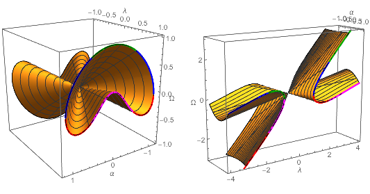
Here is another way to look at the solutions. It is not amenable to written presentation but it is a nice way to look at the problem. With a change of variables, we can transform the equation into a homogeneous polynomial poly0 of three variables. Dilations then act on the solution set and one dimension can be factored out. In other words all solutions may be obtained from scaling a given cross-section of the surface poly0 == 0.

Here are transformations for converting between poly and poly0.

homogenize = {A :> Sqrt[α]/(Sqrt[2] Pi), L -> λ/Sqrt[α], W -> Ω/Sqrt[α]};
dehomogenize = First@Solve[{A, L, W} == ({A, L, W} /. homogenize), {α, λ, Ω}]
(*
{α -> 2 A^2 π^2, λ -> Sqrt[2] A L π, Ω -> Sqrt[2] A π W}
*)

eqn0 = eqn /. homogenize // Simplify;
sols0 = Ω /. Solve[eqn0, Ω];
poly0 = Collect[5 Times @@ (Ω - sols0) // Expand // Simplify, Ω]
poly == ((W/Ω)^4 poly0 /. dehomogenize) // Expand
(*
9 α^4 - 12 α^2 λ^2 + λ^4 + (6 α^2 λ - 6 λ^3) Ω + (10 α^2 + 6 λ^2) Ω^2 - 6 λ Ω^3 + 5 Ω^4

True
*)

Any solution (for Ω or A π W) to poly0 == 0 may be obtained by dilation (scaling) of a plane section of the surface poly0 == 0. Below the relationships of each of two sections to the solution set are shown, with the mesh lines showing the dilation of the boundary curve.

sectλ = Show[
   ContourPlot3D[
    poly0 == 0, {α, -1.2, 1.2}, {λ, -1, 1}, {Ω, -1, 1},
    MeshFunctions -> {ArcTan[#1, #2] &, #2 &}, 
    PlotPoints -> 20, AxesLabel -> Automatic],
   ParametricPlot3D[
    Thread[{α, λ, sols0}] /. λ -> 1 // Evaluate, {α, -1.2, 1.2},
    PlotPoints -> 100, 
    PlotStyle -> (Directive[Thickness[0.01], #] & /@ {Red, Blue, Magenta, Darker@Green})]
   ];

sectα = Show[
   ContourPlot3D[
    poly0 == 0, {α, -1, 1}, {λ, -4, 4}, {Ω, -3, 3},
    MeshFunctions -> {ArcTan[#1, #2] &, #1 &}, PlotPoints -> 20, 
    AxesLabel -> Automatic],
   ParametricPlot3D[
    Thread[{α, λ, sols0}] /. α -> 1 // Evaluate, {λ, -4, 4},
    PlotPoints -> 100, 
    PlotStyle -> (Directive[Thickness[0.01], #] & /@ {Red, Blue, Magenta, Darker@Green})],
   BoxRatios -> {1, 4, 3}
   ];

GraphicsRow[{sectλ, sectα}]

Answer 3

Solve[L == (3 W)/2 + 3/2 Sqrt[4 A^2 Pi^2 + W^2] - Sqrt[
   6 A^2 Pi^2 + 3 W^2 + 5 W Sqrt[4 A^2 Pi^2 + W^2]]/Sqrt[2], W, 
 Quartics -> False]

or

Solve[L == (3 W)/2 + 3/2 Sqrt[4 A^2 Pi^2 + W^2] - Sqrt[
   6 A^2 Pi^2 + 3 W^2 + 5 W Sqrt[4 A^2 Pi^2 + W^2]]/Sqrt[2], W, Reals]

Answer 4

One shotgun approach is to sic Simplify or FullSimplify onto your solution:

sol1 = Solve[
   L == (3 W)/2 + (3 Sqrt[4 A^2 Pi^2 + W^2])/2 - 
     Sqrt[6 A^2 Pi^2 + 3 W^2 + 5 W Sqrt[4 A^2 Pi^2 + W^2]]/Sqrt[2], W];

sol2 = Simplify[sol1];

LeafCount /@ {sol1, sol2}
ByteCount /@ {sol1, sol2}

{3849, 3077}

{111720, 92840}

(Note: A FullSimplify attempt was stopped after several hours)

Using additional assumptions may help the simplification substantially, too.

Answer 5

Typical of questions of this type, the context and intended application can be important in shaping the "best" form for the solution.

However, one important point not made yet is that the RHS of your equation:

$L=(3W)/2+(3\sqrt(4 A^2 \pi^2+W^2))/2-\sqrt(6A^2 \pi^2+3 W^2+5 W \sqrt(4A^2 \pi^2+W^2))/\sqrt{2}$

simplifies if $A$ is re-scaled by $1/(2\pi)$ and, more importantly, that it is homogenous in $A$ and $W$—so you can also re-scale $W$ and $L$ to simplify your equation to obtain an expression for $L/W$ that only depends upon a single parameter.

And then representing the solution as "an easily-written function of $A$ and $L$" (for instance, as series expansion) is straightforward.