12
$\begingroup$

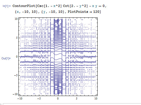
Here are several equations, it seems that Mathematica couldn't plot them well, although I set PlotPoints>100

 ContourPlot[Csc[1. - x^2] Cot[2. - y^2] - x*y == 0, 
   {x, -10, 10}, {y, -10, 10}, PlotPoints -> 120]

enter image description here

I tried

cf = Compile[{{d, _Real}}, 
   Do[If[Abs[Csc[1. - x^2] Cot[2. - y^2] - x y] < 0.02, 
     Sow@{x, y}], {x, -10, 10, d}, {y, -10, 10, d}], 
   CompilationTarget -> "C", Parallelization -> True, 
   RuntimeOptions -> "Speed"];


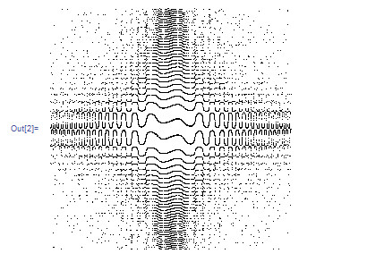
Graphics[{AbsolutePointSize@1, Point@Reap[cf[0.002]][[2, 1]]}]

but I don't know how to join the points. Is there other better method do it? enter image description here

$\endgroup$
4
  • 3
    $\begingroup$ Shouldn't there be infinities ? Compare to Plot[Csc[1 - x^2] Cot[2 - y^2] - x y /. y -> 0.5, {x, -10, 10}] for instance. $\endgroup$ Commented Feb 14, 2013 at 9:04
  • 2
    $\begingroup$ Please also post the ContourPlot code for convenience. $\endgroup$
    – Yves Klett
    Commented Feb 14, 2013 at 9:23
  • $\begingroup$ I believe the plotting routines begin by compiling their functions, anyway, so using floats and explicit compilation shouldn't yield any improvements. $\endgroup$
    – whuber
    Commented Feb 15, 2013 at 0:44
  • 1
    $\begingroup$ @whuber moreover this particular function calls out of the VM for every Sow, and such calls are very expensive (and prevent parallelization). Overall, Compile is not achieving much here and may even be net harmful. $\endgroup$ Commented Feb 15, 2013 at 1:55

4 Answers 4

15
$\begingroup$

The heart of the problem lies in the removable singularities where the cosecant or cotangent become undefined.

Recalling that $\csc(x) = 1/\sin(x)$ and $\cot(x) = \cos(x)/\sin(x)$, notice that

$$\csc(1-x^2)\cot(2-y^2) = xy$$

implies (via clearing the denominators) that

$$\cos(2-y^2) = x y \sin(1-x^2) \sin(2-y^2).$$

You can obtain this by brute force just by collecting everything into one fraction and ignoring the denominator:

Csc[1 - x^2] Cot[2 - y^2] - x y // TrigExpand // Together // Numerator // FullSimplify

$\cos \left(2-y^2\right)-x y \sin \left(1-x^2\right) \sin \left(2-y^2\right)$

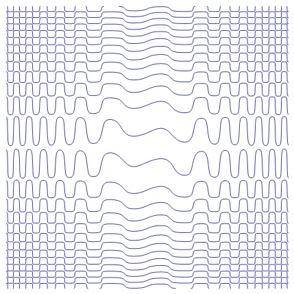
This eliminates the singularities: they are just discrete points along the contours and therefore of no consequence. Plotting it gives the desired curves. We obtain reasonable smoothness and consistency by increasing the MaxRecursion parameter; the time to make the plot is still reasonably short (under two seconds on this machine):

ContourPlot[
  Sin[1 - x^2] Sin[2 - y^2] x y - Cos[2 - y^2] == 0, {x, -2 Pi, 2 Pi}, {y, -2 Pi, 2 Pi}, 
  Frame -> None, MaxRecursion -> 3]

Figure

$\endgroup$
2
  • $\begingroup$ This is nowhere near as beautiful as @Cormullion's plot, but it's more accurate. You can use the parameters given there to create a similar-looking plot. The increased accuracy--as well as the changes wrought by clearing the denominators, which changes the values away from the contours--makes it less smooth (and less pretty) in the corners, though. $\endgroup$
    – whuber
    Commented Feb 15, 2013 at 0:38
  • 2
    $\begingroup$ If you're worried about dropping the denominator, you may compute it in a similar manner and then exclude its zeros in the plot; the option works out to Exclusions -> {Sin[1 - x^2] Sin[2 - y^2] != 0}. The resulting plot takes the same amount of time to draw and looks the same. $\endgroup$
    – whuber
    Commented Feb 15, 2013 at 0:50
17
$\begingroup$

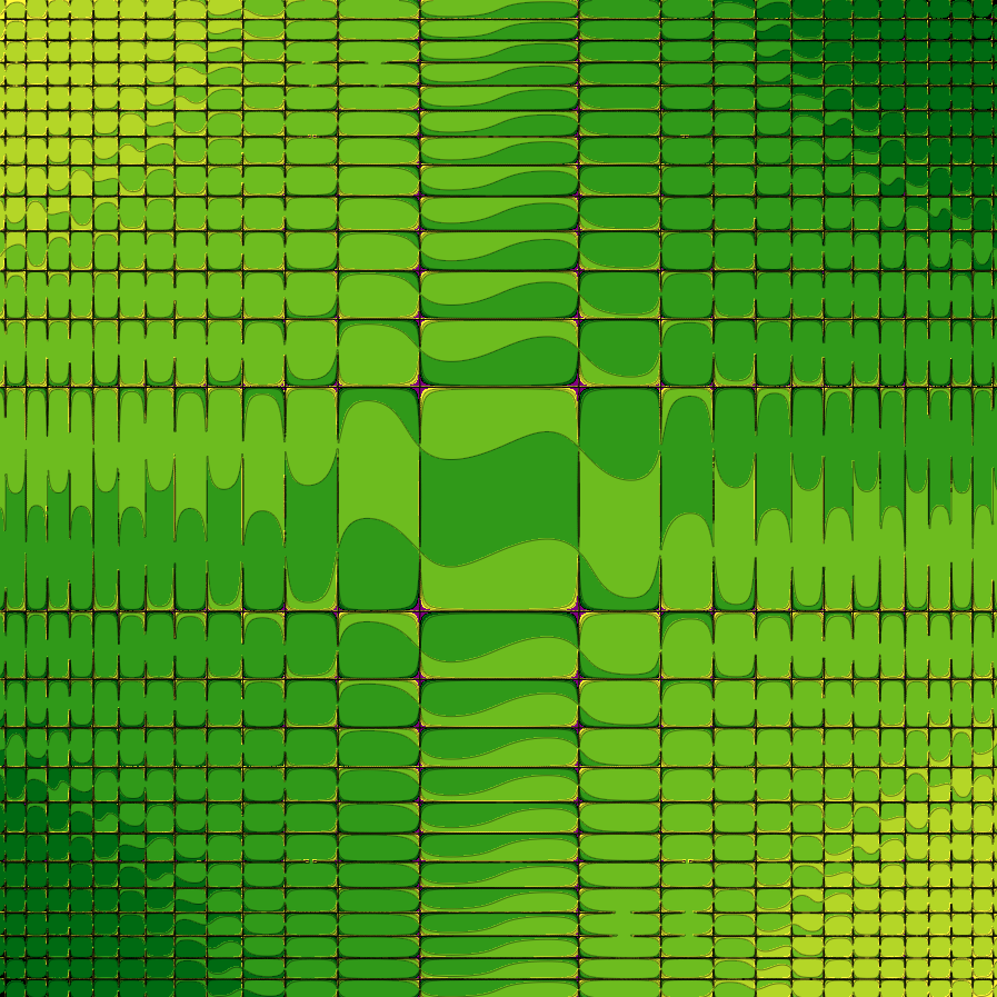
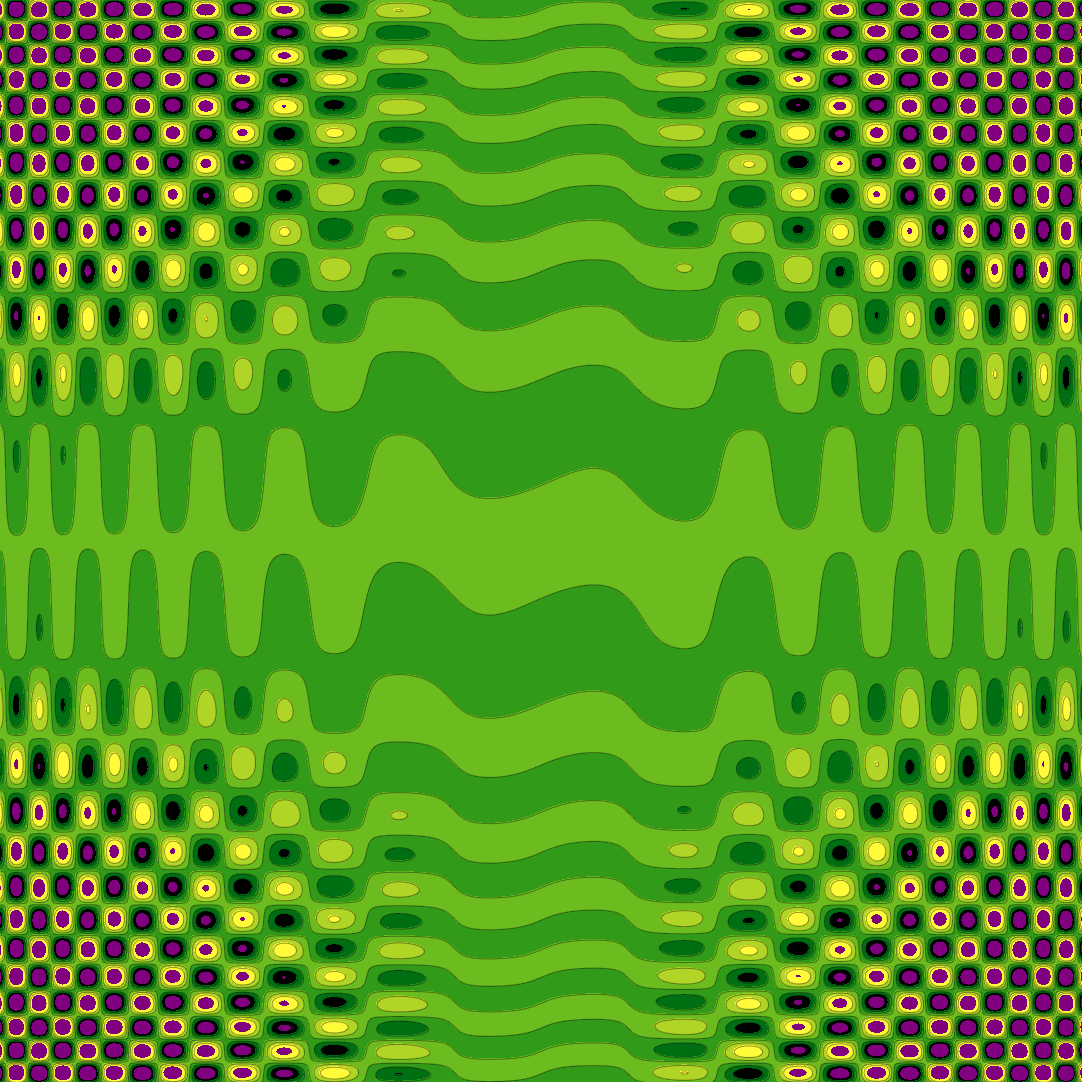
I don't know what's meant by "good" or "well", but, on the assumption that it means "like a 1970s retro wallpaper design", here's a suggestion:

retro

ContourPlot[Csc[1. - x^2] Cot[2. - y^2] - x y,
 {x, -2 Pi, 2 Pi},
 {y, -2 Pi, 2 Pi},
 ColorFunction -> "AvocadoColors",
 Frame -> None,
 MaxRecursion -> 3,
 PlotRangePadding -> None,
 Background -> Purple,
 PlotPoints -> 60]

Edit: using @whuber's excellent analysis, the design is improved - perhaps harking back to 1960's op art. (And it doesn't take 45 minutes to generate.)

retro 2

$\endgroup$
3
  • 4
    $\begingroup$ +1 I believe the key idea lies in the MaxRecursion parameter. $\endgroup$
    – whuber
    Commented Feb 14, 2013 at 18:21
  • $\begingroup$ It shows the exclusions very well. +1 $\endgroup$
    – rcollyer
    Commented Feb 14, 2013 at 20:18
  • $\begingroup$ yes, +1 for that Austin Powers flair! $\endgroup$
    – Yves Klett
    Commented Feb 15, 2013 at 14:20
9
$\begingroup$

OK, I think based on the number of times I crashed my kernel trying to reproduce that plot that brute force is not the right answer. Here's a technique that's a little more clever:

  1. Select a random point in the region of interest.
  2. Use a solver (steepest descent, say) to get onto a zero contour.
  3. Find the gradient at that point and take a vector orthogonal to it.
  4. Follow that contour until you hit a singularity or the edge of the region of interest.
  5. Goto 1, but at step 2 check whether you've landed on a contour you already solved earlier.

Here's some code that should get you started. Probably there are a lot more improvements that could be made! For example, instead of using random starting points, you could use a grid or try to find points far from your current set of lines. Or you could speed up some of the checking by using a search tree that would give only nearby lines.

Edit: New updates add a reminimization step and prune the recent line to improve performance. This allows us to lengthen the step size substantially.

Second edit: Fixed a bug in the pruning logic. Added a starting set of points to make sure the grid is reasonably well sampled.

Third edit: Added reversal along each contour so you get both directions at once. Compiled the more expensive bits. Made the starting grid more suited to the structure of the function.

Fourth edit: Minor edit to remove a v9ism (Grad).

randomzero := nearestzero[RandomReal[#] & /@ range]
nearestzero[{x0_, y0_}] := 
 Quiet[{x, y} /. FindMinimum[(f[x, y])^2, {{x, x0}, {y, y0}}][[2]]]

update := 
 Module[{}, 
  Do[x0 = If[Length[lines] < Length[initx], 
     nearestzero[initx[[Length[lines] + 1]]], randomzero]; 
   While[Min[Norm[#1 - x0] & /@ Join @@ lines] < thin step,
    x0 = randomzero];
   xlist = {x0}; cnt = -thin/2; newline = {}; Do[
    While[x1 = Last[xlist]; 
     x1[[1]] > range[[1, 1]] && x1[[2]] > range[[2, 1]] && 
      x1[[1]] < range[[1, 2]] && 
      x1[[2]] < 
       range[[2, 
        2]] && (m1 = Min[#.# &[#1 - x1] & /@ Most[xlist]]) > (step/
         1.01)^2 && (m2 = 
         If[Length[newline] == 0, 1, 
          Min[#.# &[#1 - x1] & /@ 
            Join[Sequence @@ lines, newline]]]) > (step thin/2)^2, 
     AppendTo[xlist, x1 + dir follow @@ x1]; 
     If[cnt++ == thin, AppendTo[newline, First[xlist]]; 
      xlist = Drop[xlist, thin]; 
      Block[{xtmp = Last[xlist]}, 
       ReplacePart[xlist, -1 -> nearestzero[xtmp]]; 
       If[#.# &[xtmp - Last[xlist]] > step^2, 
        Print[Norm[xtmp - Last[xlist]]]; 
        ReplacePart[xlist, -1 -> xtmp]; Break[]]]; cnt = 1;]]; 
    newline = Reverse@Join[newline, xlist[[-1 ;; ;; -thin]]]; 
    If[dir > 0, xlist = {Last[newline]}; newline = Most[newline]; 
     cnt = -thin/2], {dir, {1, -1}}];
   AppendTo[lines, newline], {Length[initx] + nadd}]; newline = {}; 
  xlist = {Last[xlist]};]

range = {{-10, 10}, {-10, 10}}; step = 0.003; thin = 30;
f[x_, y_] := Csc[1 - x^2] Cot[2 - y^2] - x y
follow = With[{orth = RotationMatrix[\[Pi]/2], 
    grad = {D[f[x, y], x], D[f[x, y], y]}}, 
   Compile[{{x, _Real}, {y, _Real}}, step orth.Normalize[grad]]];

initx = Join @@ 
  Outer[List, Join[-#, #] &@Sqrt[Range[0.5, 100, 2]], 
   Join[-#, #] &@Sqrt[Range[0.5, 100, 2]]]; lines = {}; nadd = 0;

Dynamic[Graphics[{Line[
    Append[Select[lines, Length[#] > 3 &], 
     Append[newline, First[xlist]]]], Pink, Line[xlist], Blue, 
   Point[x0], Red, Point[Last[xlist]]}, PlotRange -> range]]
update

Here's a picture of the tracer after about 4 minutes:
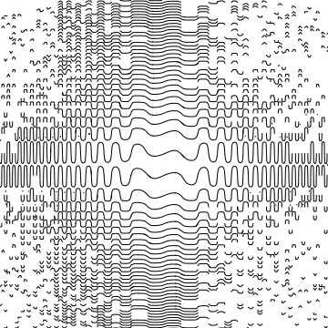
Contour tracer version 4

$\endgroup$
3
$\begingroup$

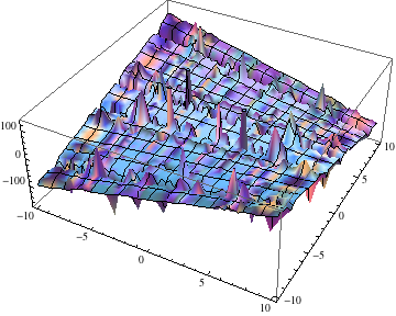
I got a plot with Mathemaica 9, but far from the one mentioned in the page you said. If one uses

Plot3D[Csc[1. - x^2] Cot[2. - y^2] - x*y, {x, -10, 10}, {y, -10, 10}]

then you get this picture:

plot3d

I don't see how a contour plot could get a region extending with similar value along the X axis as shown in the original picture when the 3D surface shows that the overall curve is a saddle.

$\endgroup$

Your Answer

By clicking “Post Your Answer”, you agree to our terms of service and acknowledge you have read our privacy policy.

Not the answer you're looking for? Browse other questions tagged or ask your own question.