You may use the [`NDSolve` Components and Data Structures](http://reference.wolfram.com/language/tutorial/NDSolveStateData.html) tutorial to control the memory usage and save down the state of intermediate runs.
Initialise the ``NDSolve`StateData`` for the complete range you need to create solutions. Below is done for `0 <= t <= 30` and I will iterate in chunks of 10.
ndsStateData = First@NDSolve`ProcessEquations[
{
D[u[t, x], t] == D[u[t, x], x, x],
u[0, x] == 0,
u[t, 0] == Sin[t],
u[t, 5] == 0
},
u,
{t, 0, 30}, {x, 0, 5}
];
Next I iterate in 3 chunks of 10. `ndsStateData` can be saved down after the current chunk's solution is extracted with ``NDSolve`ProcessSolutions``. Below I reassign `ndsStateData` with the reinitialised ``NDSolve`StateData`` instead.
sols = {};
Module[{step = #},
NDSolve`Iterate[ndsStateData, {(step - 1)*10, step 10}];
AppendTo[sols, u /. NDSolve`ProcessSolutions[ndsStateData]];
ndsStateData =
First@NDSolve`Reinitialize[ndsStateData, {u[step 10, x] == sols[[step]][step 10, x]}];
] & /@ Range@3;
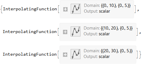
`sols` contains the 3 solutions over each chunk. Notice the difference in the domains.
sols
> 
Plotting the solutions.
Plot3D[sols[[#]][t, x], {t, (# - 1) 10, # 10}, {x, 0, 5},
PlotRange -> Full,
PlotStyle -> ColorData[109][#]
] & /@ Range@3 // Show[#, PlotRange -> All] &
> [![enter image description here][2]][2]
Hope this helps.
[1]: https://i.sstatic.net/i87GL.gif
[2]: https://i.sstatic.net/ZftqG.gif