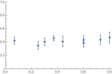
Your data:
data = {{0.067, 0.423}, {0.30, 0.408}, {0.60, 0.433}, {0.25, 0.3512}, {0.37, 0.4602}, {0.44, 0.413}, {0.60, 0.390}, {0.73, 0.437}, {0.8, 0.47}};
errors = {0.055, 0.0552, 0.0662, 0.0583, 0.0378, 0.080, 0.063, 0.072, 0.08};
ErrorListPlot[Transpose[{data, ErrorBar /@ errors}], PlotRange -> {0, 1}]
> 
Assume that the errors are distributed Normally with standard deviation given by your errors. Then we can define
diffErr[y1_, s1_, x1_, y2_, s2_, x2_] := Block[{distr, slope, error},
distr =
TransformedDistribution[(v - u)/(
x2 - x1), {u \[Distributed] NormalDistribution[y1, s1],
v \[Distributed] NormalDistribution[y2, s2]}];
slope = Mean[distr];
error = StandardDeviation[distr];
{slope, error}
]
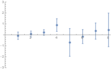
And the slopes between points ie the numerical derivative is then
slopes=Table[diffErr[data[[i, 2]], errors[[i]], data[[i, 1]], data[[i + 1, 2]], errors[[i + 1]], data[[i + 1, 1]]], {i, Length[data] - 1}]
> {{-0.0643777, 0.334435}, {0.0833333, 0.287315}, {0.233714, 0.252034}, {0.908333, 0.579016}, {-0.674286, 1.26401}, {-0.14375, 0.636427}, {0.361538, 0.735933}, {0.471429, 1.53756}}
ErrorListPlot[slopes, PlotRange -> {-3, 3}]
> 