This is a comment rather than an answer, but it grew too long for the comment box, and I wanted to show graphics, so I'll leave it here in hopes that someone better versed in the inner workings of MMA might explain this behavior. I am using your definition of the wrapper function `pp`.
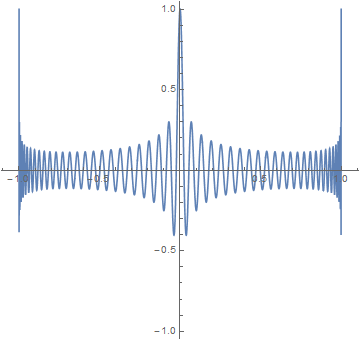
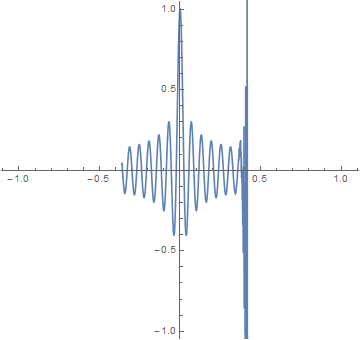
First of all, I get a **slightly different version** of the "wrong" function:

Having said that, it seems that this behavior has something to do with the **order of evaluation**. In fact, if I pass the function to plot to the `pp` wrapper *unevaluated*, then I obtain the same well-behaved output as your "free standing" `ParametricPlot`:
pp[Unevaluated@ZernikeR[100, 0, r]]

The opposite is also true: if I pre-evaluate the `ZernikeR` function, then try to plot the result, I obtain the same result I had from feeding this function straight to your wrapper:
ZernikeR[100, 0, r];
ParametricPlot[{r, %}, {r, -1, 1}, PlotRange -> {Automatic, 1.05 {-1, 1}}]

I am afraid that this is as far as I was able to go to understand the problem. Depending on how you are constructing the lists of functions to plot, you may be able to **pass the functions unevaluated programmatically**, and get around the road block for now. For instance
pp /@
Unevaluated/@
Unevaluated@
{ZernikeR[80, 0, r], ZernikeR[90, 0, r], ZernikeR[100, 0, r]}

I'd still like to understand why this is the case, however.