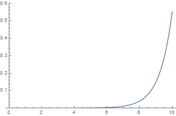
Trying using the following code. You can use three boundary values, but notice the same solution if you substitute the fourth boundary involving y'[rmax]=dmax. To this end, one of the boundaries is redundant.
c = 0.5;
rzer = 0.001;
rmax = 10.;
vmax = 0.550718236126181;
dmax = -0.032852103365844154;
sols =
   (First[
     NDSolve[{Derivative[2][y][
          r] + (1.*Csch[1.*r] - 1.25*Tanh[0.5*r]^2)*
          Derivative[1][y][
           r] + (-0.00048828125*Csch[0.5*r]^2*Sech[0.5*r]^4*
                       (14. + 139.*Cosh[1.*r] - 30.*Cosh[2.*r] +
              5.*Cosh[3.*r] + 32.*Sinh[1.*r] - 16.*Sinh[2.*r]))*y[r] ==
        0, y[rzer] == rzer, y[rmax] == vmax}, y, r,

      Method -> {"Shooting",
        "StartingInitialConditions" -> {y[rzer] == rzer,
          Derivative[1][y][rzer] == #1}}]] & ) /@ {rzer}
Plot the output using
Plot[Evaluate[y[r] /. sols], {r, rzer, rmax}, PlotRange -> {0, 0.6}]
With regard to your last answer, you can consider a second region r> 10, and then just use the last boundary condition. No need to employ the shooting method:
c = 0.5; rzer = 0.001; rmax = 10.; vmax = 0.550718236126181; dmax = \
-0.032852103365844154;
  sols2 =
 NDSolve[{Derivative[2][y][r] + (1.*Csch[1.*r] - 1.25*Tanh[0.5*r]^2)*
      Derivative[1][y][r] +
            (-0.00048828125*Csch[0.5*r]^2*
        Sech[0.5*r]^4*(14. + 139.*Cosh[1.*r] - 30.*Cosh[2.*r] +
          5.*Cosh[3.*r] + 32.*Sinh[1.*r] - 16.*Sinh[2.*r]))*y[r] == 0,
        y[rmax] == vmax, Derivative[1][y][rmax] == dmax},
  y, {r, 10, 30}]
Notice that r > = 10

