Return to Revisions

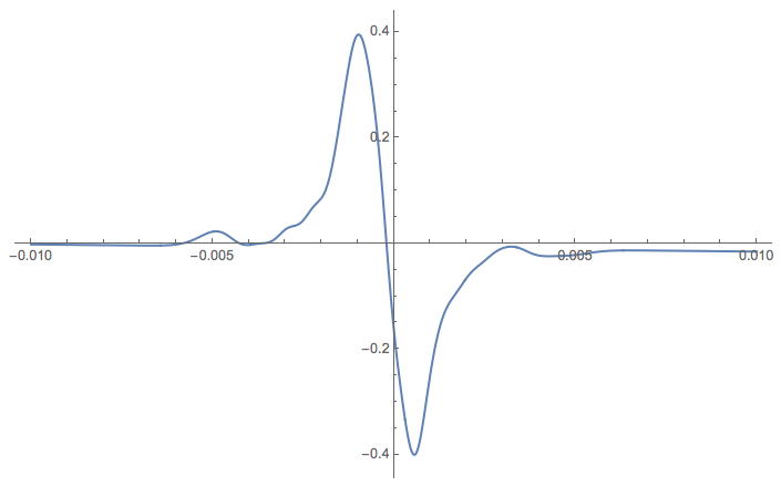
I am not sure how useful my answer is, but I hope it will bring some points to be clarified in the question. (Also I spent some time on this so I wanna proclaim some of the results of my efforts...)

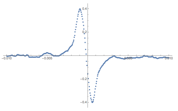
Since the data was not provided in the original question I extracted it from the image shown following the (great) explanations here: Recovering data points from an image.

Here is a plot with the extracted points:

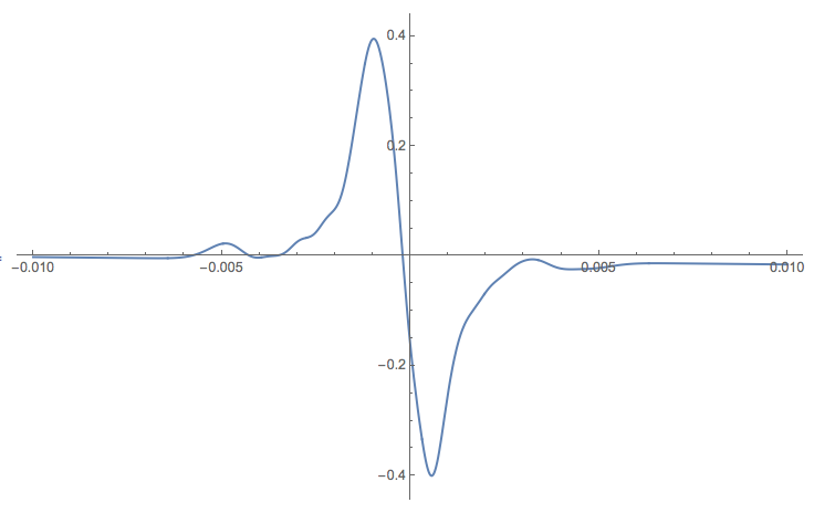
Next, I just used Chebyshev polynomials to find a fit with the following commands:

fit = Fit[data, ChebyshevT[#, 90. x] & /@ Range[0, 40], x];
Plot[fit, {x, Min[data[[All, 1]]], Max[data[[All, 1]]]}, PlotRange -> All]

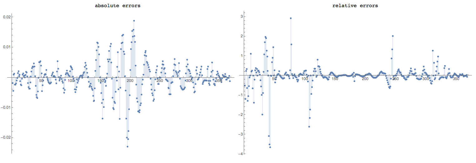
Here are the errors:

opts = {Filling -> Axis, PlotRange -> All, ImageSize -> 600};
Grid[{{"absolute errors", "relative errors"},
  {ListPlot[Map[(#[[2]] - (fit /. x -> #[[1]])) &, data], opts],
   ListPlot[
    Map[(#[[2]] - (fit /. x -> #[[1]]))/(Abs[#[[2]]] /. {0. -> 1}) &, 
     data], opts]}}]

If I understand the question correctly the fitting of a particular type of family of curves is desired. I was not able to work with the functions provided in the question. I used SkewNormalDistribution PDF that seems to have similar properties as the data. So I repeated the above commands using a generated basis of SkewNormalDistribution PDF's derived with combinations of different parameters ranges. I assume this approach would work with the functions in the question.

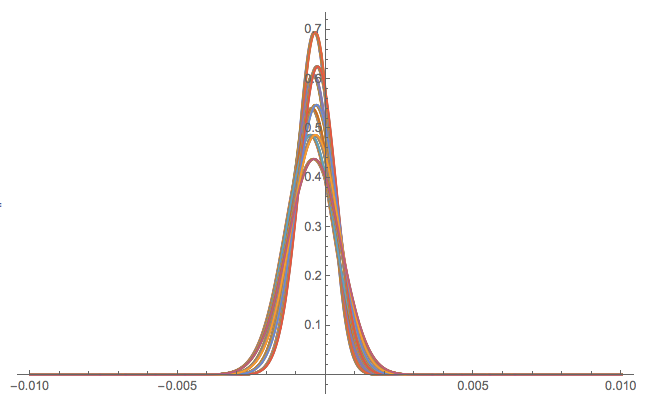
First we generate around 100 functions and plot them:

funcs = Flatten@
   Table[PDF[SkewNormalDistribution[c, s, \[Alpha]], 
      x] /. {x -> ( x*1000)}, {\[Alpha], {-1, -0.6}}, {c, -0.04, 0.01,0.004}, {s, 0.7, 1, 0.1}];
Plot[Evaluate@funcs, {x, Min[data[[All, 1]]], Max[data[[All, 1]]]}, 
 PlotRange -> All]

Note that I have chosen the peaks locations and the scale factor for x according to the peaks and spread in the experimental data.

Next using the generated functions we add to them their antisymmetric versions and {1,x,-x}. The resulted list is given to Fit:

fn = Fit[data, Join[{1, x, -x}, funcs, -funcs /. {x -> (-x)}], x];

Plot[fn, {x, Min[data[[All, 1]]], Max[data[[All, 1]]]}, 
 PlotRange -> All]

Here are the errors:

opts = {Filling -> Axis, PlotRange -> All, ImageSize -> 600};
Grid[{{"absolute errors", "relative errors"},
  {ListPlot[Map[(#[[2]] - (fn /. x -> #[[1]])) &, data], opts],
   ListPlot[
    Map[(#[[2]] - (fn /. x -> #[[1]]))/(Abs[#[[2]]] /. {0. -> 1}) &, 
     data], opts]}}]