Here the contours of a method to do this half-automatic selection you are looking for. It is heavily based on an example on the `ImageCorrelate` doc page of Waldo fame. First, you interactively select an example of the plot marker you want to look for:
img = Import["https://i.sstatic.net/hhPr9.png"];
pt = {ImageDimensions[img]/4, ImageDimensions[img]/2};
LocatorPane[
Dynamic[pt],
Dynamic[
Show[
img,
Graphics[
{
EdgeForm[Black], FaceForm[], Rectangle @@ pt
}
]
]
], Appearance -> Graphics[{Red, AbsolutePointSize[5], Point[{0, 0}]}]
]
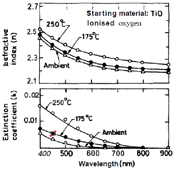
Then you use Mathematica v8's image processing tools to find similar structures:
res =
ComponentMeasurements[
MorphologicalComponents[
ColorNegate[
Binarize[
ImageCorrelate[
img,
ImageTrim[img, pt],
NormalizedSquaredEuclideanDistance
], 0.18
]
]
], {"Centroid", "Area"}, #2 > 1 & (*use only the larger hits*)
];
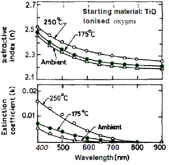
The coordinates are now in `res`. I'll show them below. Many are correct, sometimes you get some spurious hits and misses. It depends on the `Binarize` threshold value and the "Area" size chosen in `ComponentMeasurements` third argument.
Show[img, Graphics[{Green, Circle[#, 5] & /@ res[[All, 2, 1]]}]]
----
**EDIT:** Here a more complete application. It is not robust as it is (no error handling at all), but nevertheless already quite useful.
The function `getMarkers` is called with an image as argument and the name of a variable in which the final markers are returned:

You get the app with tabs that represent processing stages:
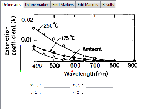
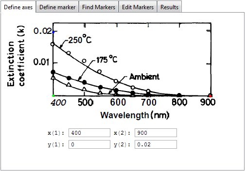
In the first tab you define the axes by dragging the colored dots to the locations on the x and y axis with the highest known value and to the origin of the plot. You also enter the values for these points here:
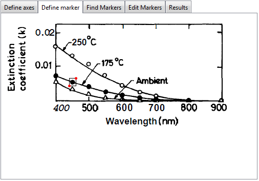
In the next tab you then indicate the marker you want to have detected:
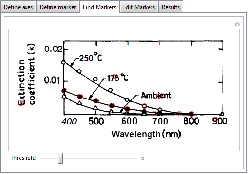
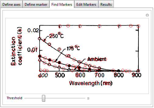
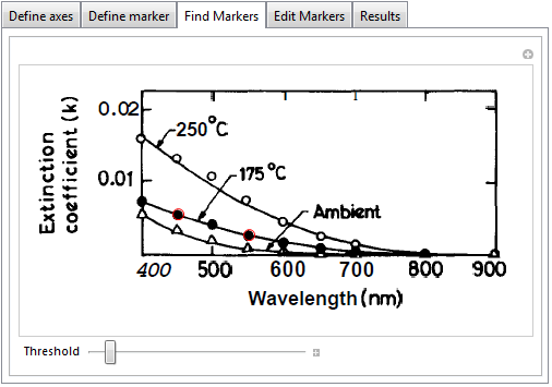
The detection results are presented in the next tab and you can drag a slider to increase or decrease the number of results:
You can manually adjust the detected markers in the next tab. Markers can be dragged, removed (alt-click an existing marker) and added (alt-click on an empty spot). Actually, this is so easy to do that I would be tempted to say that I could do without the marker-detection phase.
The end result can be seen in the Results tab. If something is wrong you can go back to an earlier tab:
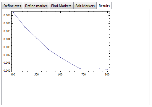.
The data plotted in the Results tab is also copied in the variable passed to the function, test in this example.
test
(*
==> {{400.5159959, 0.007353847123}, {450.3095975,
0.005511544915}, {499.8452012, 0.004129136525}, {550.9287926,
0.002664992936}, {600.4643963, 0.001702431875}, {653.869969,
0.000764540446}, {685.6037152, 0.0002398789942}, {764.7123323,
0.0002481309886}, {801.7027864, 0.0001989932135}}
*)
The code:
findMarkers[img_, pt_, thres_, minArea_] :=
ComponentMeasurements[
MorphologicalComponents[
ColorNegate[
Binarize[
ImageCorrelate[
img,
ImageTrim[img, pt],
NormalizedSquaredEuclideanDistance
], thres
]
]
], {"Centroid", "Area"}, #2 > minArea &
][[All, 2, 1]];
SetAttributes[getMarkers, HoldRest];
getMarkers[img_, resMarkers_] :=
DynamicModule[
{
pt = {ImageDimensions[img]/4, ImageDimensions[img]/2},
axisDefinePane, defineMarkerPane, findMarkerPane, editMarkersPane,
finalResultPane, xAxisBegin, xAxisEnd, yAxisBegin, yAxisEnd,
myMarkers, myTransform,
xoy = {{1/2, 1/8} ImageDimensions[img],
{1/8, 1/8} ImageDimensions[img],
{1/8, 1/2} ImageDimensions[img]}
},
axisDefinePane =
Grid[{{
LocatorPane[
Dynamic[xoy],
Dynamic[
Show[
img,
Graphics[{Line[xoy]}]
]
],
Appearance -> {Graphics[{Red, AbsolutePointSize[5],
Point[{0, 0}]}],
Graphics[{Green, AbsolutePointSize[5], Point[{0, 0}]}],
Graphics[{Blue, AbsolutePointSize[5], Point[{0, 0}]}]}
]},
{Row[{"x(1): ",
InputField[Dynamic[xAxisBegin], Number, FieldSize -> Tiny],
" x(2): ",
InputField[Dynamic[xAxisEnd], Number, FieldSize -> Tiny]}]},
{Row[{"y(1): ",
InputField[Dynamic[yAxisBegin], Number, FieldSize -> Tiny],
" y(2): ",
InputField[Dynamic[yAxisEnd], Number, FieldSize -> Tiny]}]}
}
];
defineMarkerPane =
LocatorPane[
Dynamic[pt],
Dynamic[
Show[
img,
Graphics[
{
EdgeForm[Black], FaceForm[], Rectangle @@ pt
}
]
]
],
Appearance -> Graphics[{Red, AbsolutePointSize[5], Point[{0, 0}]}]
];
findMarkerPane =
Manipulate[
Show[
img,
Graphics[{Red,Circle[#, 5] & /@ (myMarkers = findMarkers[img, pt, t, 1.05])}]
],
{{t, 0.2, "Threshold"}, 0, 1},
TrackedSymbols -> {t},
ControlPlacement -> Bottom
];
editMarkersPane =
LocatorPane[Dynamic[ myMarkers], img,
Appearance -> Graphics[{Red, Circle[{0, 0}, 1]}, ImageSize -> 10],
LocatorAutoCreate -> True
];
finalResultPane =
Dynamic[myTransform =
FindGeometricTransform[
{{xAxisEnd, yAxisBegin}, {xAxisBegin, yAxisBegin},
{xAxisBegin, yAxisEnd}
}, xoy
][[2]] // Quiet;
ListLinePlot[resMarkers = myTransform /@ Sort[myMarkers],
Frame -> True, Mesh -> All],
TrackedSymbols -> {myMarkers, xoy, xAxisEnd, yAxisBegin,
xAxisBegin, yAxisBegin, xAxisBegin, yAxisEnd}];
TabView[
{
"Define axes" -> axisDefinePane,
"Define marker" -> defineMarkerPane,
"Find Markers" -> findMarkerPane,
"Edit Markers" -> editMarkersPane,
"Results" -> finalResultPane
}
]
]