Not knowing anything else about the matrix, I can only suggest another alternative to the determinant (which sounds like it's prohibitively time-consuming).
If m is your matrix, try to find a root (or minimum) of
Min@Diagonal@SingularValueDecomposition[m][[2]]
instead. Unfortunately, SingularValueDecomposition is also very time consuming, but as I said, I don't know your matrix and therefore you may be lucky and it works. The lowest singular value will become zero when the matrix is singular.
Simplification: The second part [[2]] of SingularValueDecomposition is a square diagonal matrix, and by applying Diagonal to it I extract the one-dimensional list of singular values. This isn't really necessary since we don't need the other parts of SingularValueDecomposition. If all you want is the list of singular values, you should use
Last@SingularValueList[m]
Edit
No matter what method you end up choosing to test for the singularity of the matrix, you should probably not do it symbolically. That is, you have to define a "merit" function with your parameter $\kappa$ as a numerical variable:
Here is a crude example of a matrix and the corresponding function f:
m = {{0.7407182168539275`, 0.24672805625057825`,
   0.8493016773864293`}, {0.06662628477504584`, 0.3469746999275358`,
   0.2741493334768361`}, {0.07058419213858214`, 0.9556414582722623`,
   0.7252123775090984`}};

f[κ_?NumericQ] :=
 Last[SingularValueList[m + DiagonalMatrix[{κ, 0, 0}]]]
Edit 2: Explanation
The pattern f[κ_?NumericQ] insures that the function will return a value only if it is called with a numerical argument κ. Any minimization or root finding routine will by default attempt to simplify f[κ] symbolically, but since f is defined only for numerical arguments that attempt will fail. This is good because the automatic evaluator then chooses a purely numerical method, which in our case is faster.
The SetDelayed := in the function definition means that the evaluation on the right-hand side (i.e., the singular-value decomposition or any other decomposition you may choose) will only be performed at the time when the function is called with a numerical parameter κ. At that point, if everything else in the matrix is numerical, the entire matrix is a numerical matrix and the result will not involve anything symbolic.
Finally, the reason I take only the Last part of the SingularValueList is that it is automatically the smallest. The smallest singular value is the one that first hits zero when a matrix becomes singular. That it the point of zero determinant we're looking for.
There are complications when you work with matrices that are already close to being numerically singular, because in that case you'll have to decide how close to singular you want the matrix to get as you vary the parameter. In those cases one may have to look at the next higher singular values.
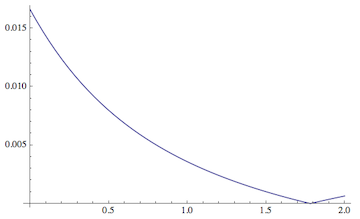
Here I plot the example f, which is now an "indicator" of how singular the matrix is:
Plot[f[κ], {κ, 0, 2}]

FindRoot[f[x], {x, 1}]

(* ==> {x -> 1.78179} *)
Applying this to your example:
f[κ_?NumericQ] :=
 Last[
   SingularValueList[{{-892.33`, 973.21`,
       44.306` + κ, -81.103`, 0}, {446.12`, -557.94`,
       0, -682.54`, -314.89`}, {0,
       893.37`, -506.68` κ, -391.457`, 0}, {0, 429.78`,
       0, -210.47`, 342.85`}, {278.32` κ, 0, 963.41`,
       217.71`, -342.68` + κ}}]]
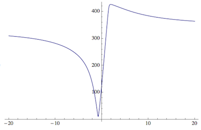
We can make a plot and realize that there won't likely be a zero for real values
κ, but in the complex plane things look more promising:
Plot[Abs[f[κ - 2 I]], {κ, -20, 20}]

Here I've subtracted an imaginary part from the real κ, and the curve seems to dip sharply down to close to zero. So let's try the following minimization:
sol = FindMinimum[Abs[f[x + I y]], {{x, -1}, {y, -2}}]
FindMinimum::lstol: The line search decreased the step size...
{1.89011*10^-6, {x -> -0.777723, y -> -2.07495}}
So there's still some work to do to get rid of the warning message, but in principle we got somewhere.
Edit 3
In order to make a pre-existing matrix mat (containing a parameter κ) into a function that you can use for root finding etc., you have to watch out for the difference between the global variable κ and the pattern instance κ that is passed to the function in place of the "dummy variable" in the pattern f[κ_?NumericQ].
The dummy variable could have equally well been named x_ or b_, so how do we make sure that it gets substituted into the matrix wherever the global variable κ appears?
Here is a way to do that. Assume the matrix is externally given as
Clear[κ]; mat = {{-892.33`, 973.21`, 44.306` + κ, -81.103`,
    0}, {446.12`, -557.94`, 0, -682.54`, -314.89`}, {0,
    893.37`, -506.68` κ, -391.457`, 0}, {0, 429.78`,
    0, -210.47`, 342.85`}, {278.32` κ, 0, 963.41`,
    217.71`, -342.68` + κ}};
Then change your function definition to
f[x_?NumericQ] := Last[SingularValueList[mat /. κ -> x]]
What this does is to replace the global κ (which you must make sure is unassigned, hence the Clear for safety) by the value of the dummy variable in the function. I have to change its name to something other than κ, so I chose x.
Edit 4
To capture what I said in some additional comments: if you do decide to use the lowest singular value as a merit function for further root finding or minimization, as a function of the parameter κ, then you may run into the problem that SingularValueList will omit the lowest singular values if they are too small relative to the largest singular value. This can lead to jumps if you plot the lowest singular value versus κ, because you aren't tracking the same singular value at all times. To insure that no singular values are omitted, one has to use
SingularValueList[m, Tolerance -> 0]
I can't answer the question of whether this is physically the best procedure, because I don't know what the physical problem is.
A very good mathematical discussion of the singular value decomposition is in Numerical Recipes in C on page 59.
