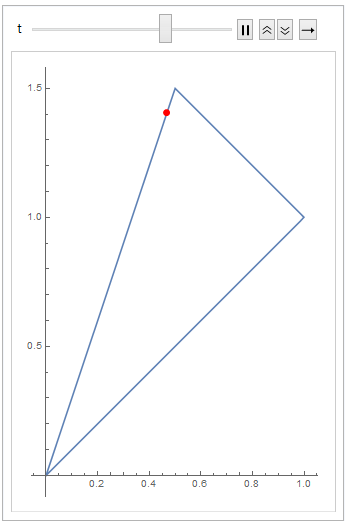
If you interpret your geometric shape as NURBS of degree 1 (linear), you can proceed with the following, extremely simple code:
pts={{0, 0},{1, 1},{0.5, 1.5}}; (* just an example *)
s=BSplineFunction[pts,SplineClosed->True,SplineDegree->1];
Animate[ParametricPlot[s[t],{t,0,1},Epilog:>{Red,PointSize[Large],Point[s[t]]}],{t, 0., 1.}]
This yields:

Just replace Animate by Manipulate to give the user control over the point.
Note This is a rather general approach applicable in wide areas, since you can vary your control points as well as the spline degree, but the BSplineFunction will always yield the curve between arguments 0 and 1. In essence, you can display quite every geometric shape using this approach. For more complex ones, some adjustment to BSpline-weights will be necessary, though.
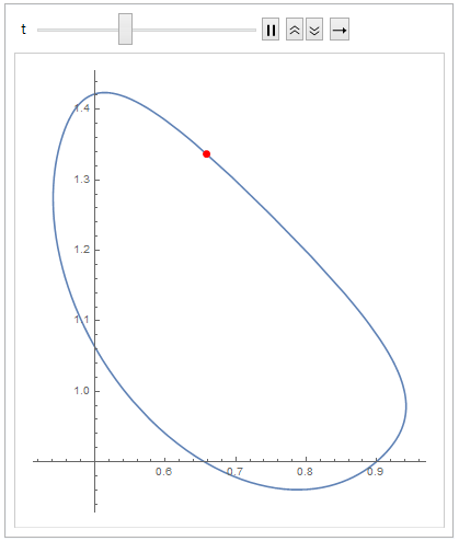
Here the curve with the same control points as before, but degree 2 and weights explicitly given as SplineWeights -> {.1, 1, 1} (please also note the change in the plotted range). Just exchange the s-line above with this one:
s = BSplineFunction[pts, SplineClosed -> True, SplineDegree -> 2, SplineWeights -> {.1, 1, 1}];

I hope this might be of some help to you.
