Below are some techniques that together with @nikie answer give you a powerful way of detecting specific table grids.
The Rubber Band Algorithm
=========================
The 3 columns to be detected must be very close to 40%, 15% and 45% of the total table width. Similarly, the line heights have a proportion to follow. So the first problem to solve is how to identify a sequence that matches a proportions pattern.
I first tried to look for a _Mathematica_ built-in function as this is a very generic task. The closest I could find is the `SequenceAlignment` function but it work only on strings. So I developed my own algorithm which is explained in this [video](http://www.youtube.com/watch?v=d_FntrHdRyY)
This is how I implemented it:
rubberBandComparePair[wanted_List, suspectsSubset_List] :=
Module[{rubberBand, reducedSuspects},
rubberBand = Rescale[wanted,
{ Min@wanted , Max@wanted },
{ Min@suspectsSubset, Max@suspectsSubset }];
reducedSuspects = If[Length @ rubberBand < Length @ suspectsSubset,
Flatten[Nearest[suspectsSubset, #] & /@ rubberBand],
suspectsSubset];
{EuclideanDistance[rubberBand, reducedSuspects] /
(Max@reducedSuspects - Min@reducedSuspects),
reducedSuspects}
] /; Length@wanted <= Length@suspectsSubset
rubberBandCompare[wanted_List, suspects_List] :=
Module[{w, k = Length @ wanted, costs, sortedSuspects},
sortedSuspects = Union @ Sort @ suspects;
w = Length @ sortedSuspects;
costs = Flatten[#, 1] & @
Table[rubberBandComparePair[wanted, sortedSuspects[[start ;; end]]],
{start, 1, w - k + 1},
{end, start + k - 1, w}];
SortBy[costs, First][[1]]
] /; Length @ Union @ suspects >= Length @ wanted
rubberBandCompare[wanted_List, suspects_List] :=
{∞, {}} /; Length[Union@suspects] < Length[wanted]
For example if we are looking for a sequence proportional to {1,2,4} in the list {9, 10, 15, 21, 40, 55}:
In[1] = rubberBandCompare[{1, 2, 4}, {9, 10, 15, 21, 40, 55}]
Out[1] = {1/30, {10, 21, 40}}
and we have detected that {10,21,40} matches {1,2,4} with an error of 1/30. Notice that this error is a relative error that does not change with scale:
In[2] = rubberBandCompare[{1, 2, 4}, {90, 100, 150, 210, 400, 550}]
Out[2] = {1/30, {100, 210, 400}}
Detecting horizontal and vertical lines
=======================================
In order to detect lines we can use `ImageLines[]` or we can use the lower lever `Radon[]`. The advantage of `ImageLines` is that it is fast and simple, but it always looks for lines in all directions whereas `Radon` lets you look for lines in a specific direction. I implemented solutions using both, but I'll explain here only the ImageLines[] solution which worked well in a large number of cases.
`ImageLines` returns a list of lines where each line is defined by 2 points. So we first write this very simple function to calculate the angle of a line:
lineAngle::usage = "lineAngle[{{x1,y1},{x2,y2}}] returns the angle of the line that goes
through points {x1,y1} and {x2,y2}.";
lineAngle[{{ x_?NumericQ, y_?NumericQ},{x_ , y_ }}]:=Indeterminate
lineAngle[{{ x_?NumericQ,y1_?NumericQ},{x_ , y2_?NumericQ}}]:=Pi/2
lineAngle[{{x1_?NumericQ,y1_?NumericQ},{x2_?NumericQ, y2_?NumericQ}}]:=ArcTan[(y2-y1)/(x2-x1)]
When we call ImageLines later on, it will return a list of lines, so we need a function to select the ones that are close to the desired direction. For this I wrote this function:
selectLinesNearAngle::usage =
"selectLinesNearAngle[{{{x1,y1},{x2,y2}},...}, angle, tolerance] \
selects the lines that have an inclination of angle +/- tolerance. \
Each line is defined by a pair of points.";
selectLinesNearAngle[lines_List, angle_?NumericQ, angularTolerance:(_?NumericQ): 4°] :=
Select[
lines,
Or @@ Thread[Abs[lineAngle[#] - angle + {-Pi, 0, Pi}] < angularTolerance] &]
Now we are ready to write our modified version of `ImageLines` for horizontal or vertical lines:
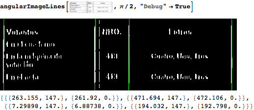
Options[angularImageLines] = {"Debug" -> False};
angularImageLines[img_Image, α_, OptionsPattern[]]:=
Module[
{lines, selectedLines, binarizedImage},
binarizedImage = Binarize@GaussianFilter[img, 3, Switch[α, 0, {2,0}, Pi/2, {0,2}]];
lines = ImageLines[binarizedImage];
selectedLines = selectLinesNearAngle[lines,α];
If[OptionValue["Debug"],
Print[Show[binarizedImage, Epilog -> {Green, Line /@ selectedLines}]]];
selectedLines
]/; α==0 || α==Pi/2
Notice that `binarizedImage` is using GaussianFilters as @nikie recommends. This is an example of how it works:

Searching for the lines that match wanted proportions
=====================================================
It is now the time to use `rubberBandCompare` and `angularImageLines` together:
matchedLines[wanted_List, g_Image, α_] :=
Module[
{candidateSequence, suspects, error, bestMatch, lines},
lines = angularImageLines[g, α];
suspects = Sort[Switch[α, Pi/2, First, 0, Last] /@ ((#1[[1]] + #1[[2]])/2 & ) /@ lines];
candidateSequence = rubberBandCompare[wanted, suspects];
If[Head[candidateSequence] === rubberBandCompare, Return[$Failed]];
{error, bestMatch} = candidateSequence;
If[α == Pi/2 && error > 0.01176495, Return[$Failed]];
If[α == 0 && error > 0.02994115, Return[$Failed]];
(Cases[lines, {{x1_, y1_}, {x2_, y2_}} /;
Switch[α, Pi/2, (x1+x2)/2, 0, (y1+y2)/2] == #1, 1, 1][[1]] & ) /@ candidateSequence[[2]]
]
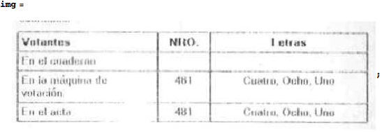
Notice that the error needs to be lower than a calibration constant for the solution to be accepted. These constants are found using a set of sample files, and making a histogram of the errors.
This is an example:

Lines Intersections
===================
This function finds the intersection of two lines. It was found in the `PlaneGeometry.m` package by Eric Weisstein (see <http://mathworld.wolfram.com/Line-LineIntersection.html>):
Intersections[Line[{{x1_, y1_}, {x2_, y2_}}],
Line[{{x3_, y3_}, {x4_, y4_}}]] :=
Module[
{d = (x1-x2) * (y3-y4) - (x3-x4) * (y1-y2),
d12 = Det[{{x1, y1}, {x2, y2}}],
d34 = Det[{{x3, y3}, {x4, y4}}]},
If[NumericQ[d] && d == 0.,
PointAtInfinity,
{Det[ {{d12, x1-x2}, {d34, x3-x4}} ]/d,
Det[ {{d12, y1-y2}, {d34, y3-y4}} ]/d}]
]
Uniformize Background
=====================
This technique is explained by @nikes [here](http://dsp.stackexchange.com/questions/1932/what-are-the-best-algorithms-for-document-image-thresholding-in-this-example/1934#1934). I just added the `/.0. -> 0.0001` in order to avoid division by zero when large pure black areas are present:
uniformizeBackground[g_Image] := Image[ImageData[g]/(ImageData[Closing[g, DiskMatrix[5]] /. 0. -> 0.0001)]
Grid Centers
============
gridCenters[g_Image] :=
Module[
{gAdjusted, hLines, vLines,
wantedX = {16.5, 224.5, 302.5, 535.5},
wantedY = {22.5, 50.5, 97.5, 125.5, 154.5}},
gAdjusted = uniformizeBackground[g];
{hLines, vLines} = {{wantedY, 0}, {wantedX, Pi/2}} /.
{wanted_List, (α_)?NumericQ} :> matchedLines[wanted, gAdjusted, α, opts];
If[hLines == $Failed || vLines == $Failed, Return[$Failed]];
Outer[Intersections, Line /@ hLines, Line /@ vLines]
]
The `wantedX` and `wantedY` are found from a sample image using the get coordinates tool from the drawing tools palette.
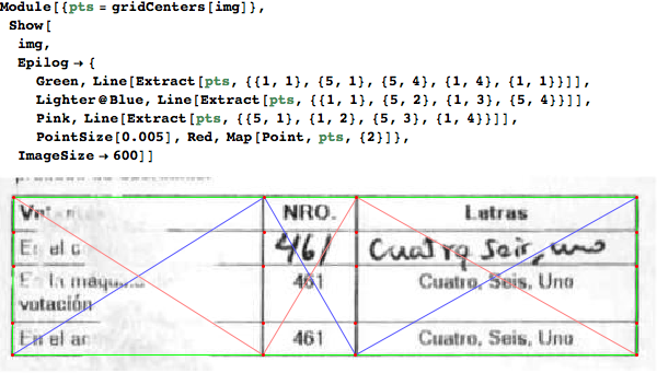
Once we have the grid centers, we can use the same techniques that @nikie used to identify and straighten any of the cells.
This is an example:


A final comment
===============
My main contribution in this answer in the rubberBandCompare function which useful to other people in other areas. If it was already invented somewhere else, please let me know.