Here is the example from the documentation adapted for the OP's data:
data = MapIndexed[
   Flatten[{#2, #1}] &,
   {2, 5, 9, 15, 22, 33, 50, 70, 100, 145, 200, 280, 375, 495, 635, 800,
    1000, 1300, 1600, 2000, 2450, 3050, 3750, 4600, 5650, 6950}];
f = Interpolation@data
(* InterpolatingFunction[{{1, 26}}, <>] *)
pwf = Piecewise[
     Map[{InterpolatingPolynomial[#, x], x < #[[3, 1]]} &, Most[#]],
     InterpolatingPolynomial[Last@#, x]] &@Partition[data, 4, 1];
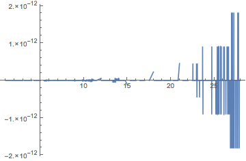
Here is a comparison of the piecewise interpolating polynomials and the interpolating function:
Plot[f[x] - pwf, {x, 1, 28}, PlotRange -> All]

The values of f[27] and f[28] are beyond the domain, which is 1 <= x <= 26, and extrapolation is used. The formula for extrapolation is given by the last InterpolatingPolynomial in pwf:
Last@pwf
(* 3750 + (850 + (100 + 25/3 (-25 + x)) (-24 + x)) (-23 + x) *)
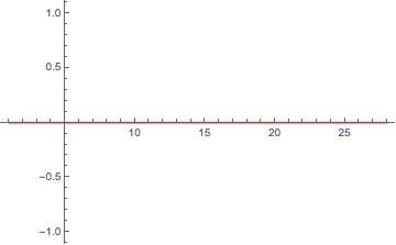
In response to a comment: The error in the plot has to do with round-off error. Apparently the calculation done by InterpolatingFunction, while algebraically equivalent, is not numerically identical. The error was greatest above in the domain 26 < x < 28 where extrapolation is performed. With arbitrary precision, the error is zero, as shown below.
Plot[f[x] - pwf, {x, 1, 28}, PlotRange -> All,
 WorkingPrecision -> $MachinePrecision, Exclusions -> None, PlotStyle -> Red]

