I'm trying to numerically solve a system of Shallow Water Equations in Wolfram Mathematica 14.0.0 on the rotating sphere by using the NDSolve method with a purpose of earthquake-generated Tsunami simulation. I define necessary physical constants, initial ocean floor profile, initial values of angular speeds and water surface. I also setup time-dependent ocean floor excitation law and atmospheric pressure function.

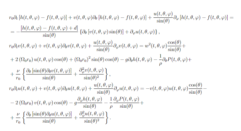
Shallow Water Gravity Waves Equations are presented below: Here are my code cuttings:

r0 = 6.4*10^6; (*Earth radius*)
g = 9.81; (*Earth gravitational constant*)
\[Omega]0 = 7.3*10^-5; (*Earth angular speed*)
\[Omega]0 = 0; (*set in order to simplify problem visualization*)
d = 10^4; (*average depth of ocean between surface and floor*)
p0 = 1.013*10^5; (*normal atmospheric pressure*)
\[Rho] = 10^3; (*water normal density*)
\[Nu] = 1.003*10^-6; (*water normal kinematic viscosity*)

\[Theta]min = 0 + \[Pi]/10;
\[Theta]max = \[Pi] - \[Pi]/10;
\[Phi]min = 0;
\[Phi]max = 2 \[Pi];

FloorProfile[\[Theta]_, \[Phi]_] := 
  d/4*Sin[2 \[Theta]]*(1 + 1/2 Sin[\[Phi]]);
Compensator[\[Theta]_, \[Phi]_] := 
  1/(2*g)*(\[Omega]0*r0)^2*Sin[\[Theta]]^2;

\[Theta]exmin = 0.45*\[Pi];
\[Theta]exmax = 0.55*\[Pi];
\[Phi]exmin = 0.95*\[Pi];
\[Phi]exmax = 1.05*\[Pi];
aex = d/100;
tex = 10;

FloorProfileExcitation[t_, \[Theta]_, \[Phi]_] := 
  If[t <= 0, 0, If[t >= tex, aex, aex/tex*t]]*
   If[\[Theta]exmin < \[Theta] < \[Theta]exmax, 
    Sin[\[Pi]*((\[Theta] - \[Theta]exmin)/(\[Theta]exmax - \
\[Theta]exmin))]^2, 0]*
   If[\[Phi]exmin < \[Phi] < \[Phi]exmax, 
    Sin[\[Pi]*((\[Phi] - \[Phi]exmin)/(\[Phi]exmax - \
\[Phi]exmin))]^2, 0];

f[t_, \[Theta]_, \[Phi]_] := 
  FloorProfile[\[Theta], \[Phi]] + 
   FloorProfileExcitation[t, \[Theta], \[Phi]];
p[t_, \[Theta]_, \[Phi]_] := p0;
h0[\[Theta]_, \[Phi]_] := Compensator[\[Theta], \[Phi]];
v0[\[Theta]_, \[Phi]_] := 0;
u0[\[Theta]_, \[Phi]_] := 0;

tsim = 10^5;

equations = {r0*\!\(
\*SubscriptBox[\(\[PartialD]\), \(t\)]\((h[t, \ \[Theta], \ \[Phi]] - 
         f[t, \ \[Theta], \ \[Phi]])\)\) + 
     v[t, \[Theta], \[Phi]]*\!\(
\*SubscriptBox[\(\[PartialD]\), \(\[Theta]\)]\((h[
          t, \ \[Theta], \ \[Phi]] - f[t, \ \[Theta], \ \[Phi]])\)\) +
      u[t, \[Theta], \[Phi]]*\!\(
\*SubscriptBox[\(\[PartialD]\), \(\[Phi]\)]\((h[
          t, \ \[Theta], \ \[Phi]] - f[t, \ \[Theta], \ \[Phi]])\)\)/
      Sin[\[Theta]] + (h[t, \[Theta], \[Phi]] - 
        f[t, \[Theta], \[Phi]] + d)*(\!\(
\*SubscriptBox[\(\[PartialD]\), \(\[Theta]\)]\((v[
            t, \ \[Theta], \ \[Phi]]*Sin[\[Theta]])\)\) + \!\(
\*SubscriptBox[\(\[PartialD]\), \(\[Phi]\)]\(u[
          t, \ \[Theta], \ \[Phi]]\)\))/Sin[\[Theta]] == 0, r0*\!\(
\*SubscriptBox[\(\[PartialD]\), \(t\)]\(v[
        t, \ \[Theta], \ \[Phi]]\)\) + v[t, \[Theta], \[Phi]]*\!\(
\*SubscriptBox[\(\[PartialD]\), \(\[Theta]\)]\(v[
        t, \ \[Theta], \ \[Phi]]\)\) + u[t, \[Theta], \[Phi]]*\!\(
\*SubscriptBox[\(\[PartialD]\), \(\[Phi]\)]\(v[
        t, \ \[Theta], \ \[Phi]]\)\)/Sin[\[Theta]] == 
    u[t, \[Theta], \[Phi]]^2*Cos[\[Theta]]/Sin[\[Theta]] + 
     2*\[Omega]0*r0*u[t, \[Theta], \[Phi]]*
      Cos[\[Theta]] + (\[Omega]0*r0)^2 Sin[\[Theta]]*Cos[\[Theta]] - 
     g*\!\(
\*SubscriptBox[\(\[PartialD]\), \(\[Theta]\)]\(h[
        t, \ \[Theta], \ \[Phi]]\)\) - 1/\[Rho]*\!\(
\*SubscriptBox[\(\[PartialD]\), \(\[Theta]\)]\(p[
        t, \ \[Theta], \ \[Phi]]\)\) + \[Nu]/r0*( \!\(
\*SubscriptBox[\(\[PartialD]\), \(\[Theta]\)]\((Sin[\[Theta]]*\ 
\*SubscriptBox[\(\[PartialD]\), \(\[Theta]\)]v[
             t, \ \[Theta], \ \[Phi]])\)\)/Sin[\[Theta]] + \!\(
\*SubscriptBox[\(\[PartialD]\), \(\[Phi]\)]\(
\*SubscriptBox[\(\[PartialD]\), \(\[Phi]\)]v[
           t, \ \[Theta], \ \[Phi]]\)\)/Sin[\[Theta]]^2), r0*\!\(
\*SubscriptBox[\(\[PartialD]\), \(t\)]\(u[
        t, \ \[Theta], \ \[Phi]]\)\) + v[t, \[Theta], \[Phi]]*\!\(
\*SubscriptBox[\(\[PartialD]\), \(\[Theta]\)]\(u[
        t, \ \[Theta], \ \[Phi]]\)\) + u[t, \[Theta], \[Phi]]*\!\(
\*SubscriptBox[\(\[PartialD]\), \(\[Phi]\)]\(u[
        t, \ \[Theta], \ \[Phi]]\)\)/
      Sin[\[Theta]] == -v[t, \[Theta], \[Phi]]*u[t, \[Theta], \[Phi]]*
      Cos[\[Theta]]/Sin[\[Theta]] - 
     2*\[Omega]0*r0*v[t, \[Theta], \[Phi]]*Cos[\[Theta]] - g*\!\(
\*SubscriptBox[\(\[PartialD]\), \(\[Phi]\)]\(h[
        t, \ \[Theta], \ \[Phi]]\)\)/Sin[\[Theta]] - 1/\[Rho]*\!\(
\*SubscriptBox[\(\[PartialD]\), \(\[Phi]\)]\(p[
        t, \ \[Theta], \ \[Phi]]\)\)/Sin[\[Theta]] + \[Nu]/r0*( \!\(
\*SubscriptBox[\(\[PartialD]\), \(\[Theta]\)]\((Sin[\[Theta]]*\ 
\*SubscriptBox[\(\[PartialD]\), \(\[Theta]\)]u[
             t, \ \[Theta], \ \[Phi]])\)\)/Sin[\[Theta]] + \!\(
\*SubscriptBox[\(\[PartialD]\), \(\[Phi]\)]\(
\*SubscriptBox[\(\[PartialD]\), \(\[Phi]\)]u[
           t, \ \[Theta], \ \[Phi]]\)\)/Sin[\[Theta]]^2)};


initialconditions1 = {h[0, \[Theta], \[Phi]] == h0[\[Theta], \[Phi]], 
   v[0, \[Theta], \[Phi]] == v0[\[Theta], \[Phi]], 
   u[0, \[Theta], \[Phi]] == u0[\[Theta], \[Phi]], 
   PeriodicBoundaryCondition[
    h[t, \[Theta], \[Phi]], \[Phi] == 2*\[Pi], 
    TranslationTransform[{0, -2*\[Pi]}]], 
   PeriodicBoundaryCondition[
    v[t, \[Theta], \[Phi]], \[Phi] == 2*\[Pi], 
    TranslationTransform[{0, -2*\[Pi]}]], 
   PeriodicBoundaryCondition[
    u[t, \[Theta], \[Phi]], \[Phi] == 2*\[Pi], 
    TranslationTransform[{0, -2*\[Pi]}]], 
   PeriodicBoundaryCondition[h[t, \[Theta], \[Phi]], \[Phi] == 0, 
    TranslationTransform[{0, 2*\[Pi]}]], 
   PeriodicBoundaryCondition[v[t, \[Theta], \[Phi]], \[Phi] == 0, 
    TranslationTransform[{0, 2*\[Pi]}]], 
   PeriodicBoundaryCondition[u[t, \[Theta], \[Phi]], \[Phi] == 0, 
    TranslationTransform[{0, 2*\[Pi]}]]}; 
method1 = 
  Method -> {"PDEDiscretization" -> {"MethodOfLines", 
      "TemporalVariable" -> t, 
      "SpatialDiscretization" -> {"FiniteElement", 
        "MeshOptions" -> {"MeshElementType" -> "TriangleElement"}}}};
region1 = {\[Theta], \[Phi]} \[Element] 
   Rectangle[{\[Theta]min, \[Phi]min}, {\[Theta]max, \[Phi]max}];

initialconditions2 = {h[0, \[Theta], \[Phi]] == h0[\[Theta], \[Phi]], 
   v[0, \[Theta], \[Phi]] == v0[\[Theta], \[Phi]], 
   u[0, \[Theta], \[Phi]] == u0[\[Theta], \[Phi]], 
   h[t, \[Theta], 0] == h[t, \[Theta], 2 \[Pi]], 
   v[t, \[Theta], 0] == v[t, \[Theta], 2 \[Pi]], 
   u[t, \[Theta], 0] == u[t, \[Theta], 2 \[Pi]]};
method2 = 
  Method -> {"PDEDiscretization" -> {"MethodOfLines", 
      "TemporalVariable" -> t, 
      "SpatialDiscretization" -> {"TensorProductGrid", 
        "DifferenceOrder" -> "Pseudospectral"}}};
region2 = 
  Sequence @@ {{\[Theta], \[Theta]min, \[Theta]max}, {\[Phi], \
\[Phi]min, \[Phi]max}};

initialconditions3 = {h[0, \[Theta], \[Phi]] == h0[\[Theta], \[Phi]], 
   v[0, \[Theta], \[Phi]] == v0[\[Theta], \[Phi]], 
   u[0, \[Theta], \[Phi]] == u0[\[Theta], \[Phi]]};
method3 = Method -> Automatic;

RunNDSolveValue[opts___] := 
  NDSolveValue[{equations, initialconditions1}, {h, v, u}, {t, 0, 
    tsim}, region1, MaxSteps -> 5000, 
   MaxStepSize -> 50, StartingStepSize -> 1, 
   InterpolationOrder -> All, AccuracyGoal -> Automatic, method1, 
   PrecisionGoal -> Automatic, opts];
Module[{time = 
     0}, (Monitor[
      solution = RunNDSolveValue[StepMonitor :> (time = t)], 
      ProgressIndicator[time/tsim]];)]; // AbsoluteTiming

My WM implementation code with plots and some other metadata was uploaded on my Google Drive.

In general, I need to simulate wave propagation on a very specific domain (world-wide ocean landscape) with periodic boundary conditions over latitude.

According to the post, my case could be evaluated only with FiniteElement method (FEM). As it was shown in @SantaP's answer under the post (thanks @xzczd for link), I ought to use PeriodicBoundaryCondition with "MeshOptions" -> {"MeshElementType" -> "TriangleElement"} option for FEM in order to obtain stable correct solution.

So, my first toy model is expressed via initialconditions1 & method1 & region1 parameters for RunNDSolveValue function.

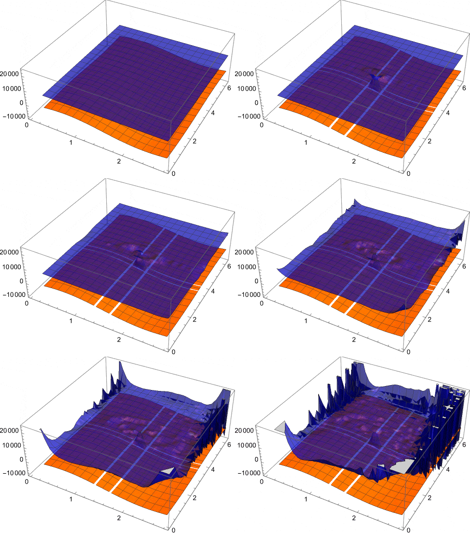
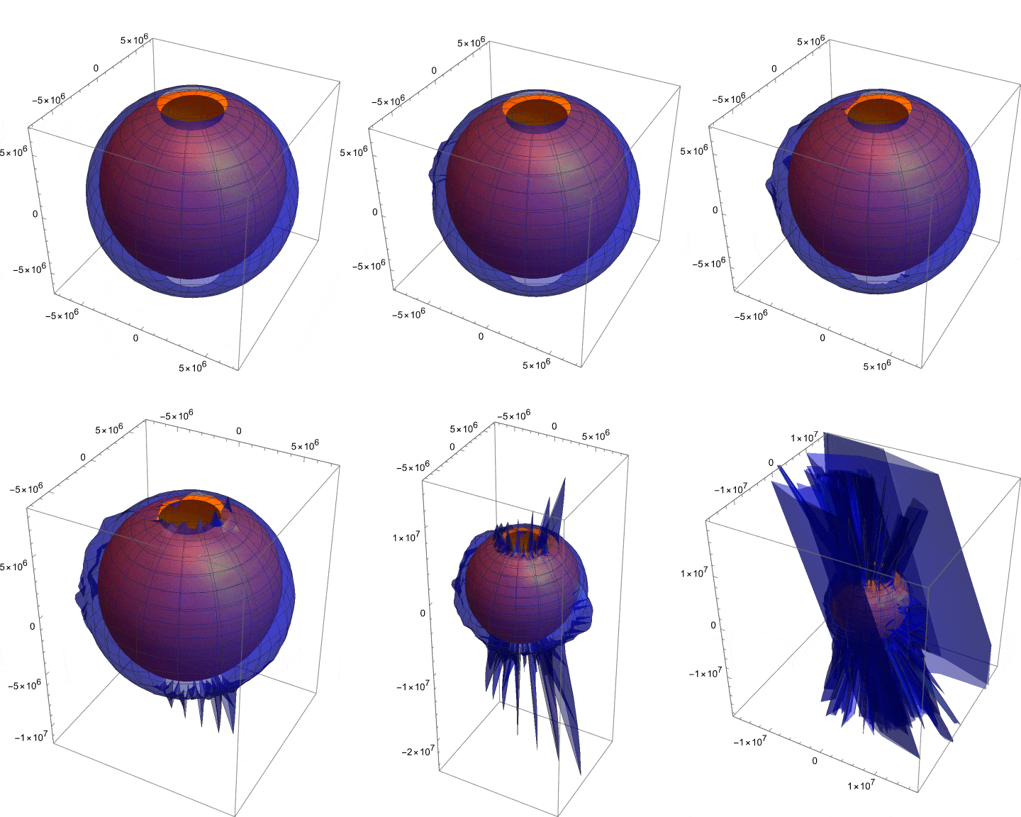
However, at some point of simulation I always receive an error "At t == ~18000, step size is effectively zero; singularity or stiff system suspected." When I try to visualize my solution, I also see that it tends to rapidly burst after some iterations. One could see my problem on the animated video below:

Being frustrated about FEM's accuracy by the discussion, I've tried to play with "SpatialDiscretization" -> {"TensorProductGrid", "DifferenceOrder" -> "Pseudospectral"} as it was recommended in the post. This attempt corresponds to initialconditions2 & method2 & region2 parameters for RunNDSolveValue function. Boundary conditions are still periodic here, but further complexification of the spatial domain is unavailable. Unfortunately, this hopeful scheme also crashes with the same error "At t == ~1200, step size is effectively zero; singularity or stiff system suspected." and new warning "An insufficient number of boundary conditions have been specified for the direction of independent variable [Theta]. Artificial boundary effects may be present in the solution."

Moreover, the most trivial default technique initialized with initialconditions3 & method3 & region2 parameters for RunNDSolveValue has the similar behaviour.

Furthermore, I’ve also googled some other different options for NDSolveValue function from here and here, but none of them helped me to stabilize calculation process near the boundary of the simulation region. At the small simulation times I can clearly see my tsunami propagating correctly. In contrast, at the large times numerical interpolation solution explodes with enormous water surface height values without any reason.

So, give me, please, some advice how to deal with such issue. I’m out of ideas ☹