Let's first test which distribution is more likely.
FindDistribution[data[[All, 2]], 5, All]
 What I did was ignore the binning with the command data[[All, 2]], and doing that doesn't really harm anything other than shift the data by about 23 to the left. This shows us that a normal distribution is likely good enough, and it would take a 3 parameter Weibull distribution to be competitive. Now this may be a three parameter Weibull distribution. In any case, treating it like a normal distribution one can
f1 = FindFit[data,c0 PDF[NormalDistribution[mu,sigma], x], {{c0, 1}, {mu, 23}, {sigma, 0.11}}, x]
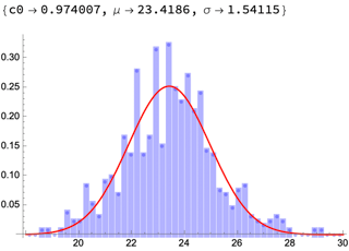
Show[ListPlot[data, Filling -> Axis, FillingStyle -> Thickness[0.018],PlotStyle -> Directive[Blue, Opacity[.3]]], Plot[Evaluate[c0 PDF[NormalDistribution[mu, sigma], x] /. f1], {x, 18, 30}, PlotStyle -> Red]]
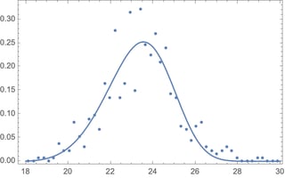
Which shows the data with its fit function. There is likely some skewness, so one could try a three parameter Weibull distribution. Given the magnitude of the $x$-values, without a location parameter, I don't think a two-parameter Weibull would work as well.
Edit Worrying about ML or not ML is not a first consideration. Before that let's further examine which distribution is in play. So how did Sjoerd C. de Vries, in his answer, know to try a three parameter Weibull distribution other by doing something like I did above? Here is another way of showing a three parameter Weibull.
fit=NonlinearModelFit[data2,kk PDF[WeibullDistribution[a0,a1,a2],x],{kk,a0,a1,a2},x,WorkingPrecision->30,MaxIterations->1000];
Show[ListPlot[data2],Plot[fit[x],{x,18,30}],Frame->True]
fit["BestFitParameters"]
{kk->0.964661496866093819527120602321,a0->4.72300143536200858818774078537,a1->6.80075698971527535007544086964,a2->17.0803838666758819512633107980}
Further steps are to model the data as is, e.g., with a Poisson loss function as it is count data (see JimB's answer) and note that we haven't proven anything here. We still need to test distributions for goodness of fit to gain more insight.
Also note this post https://mathematica.stackexchange.com/a/104279/42558, which includes
(* GerneralizedLinearModelFit - logically the same as maximum
likelihood estimate *)
glm = GeneralizedLinearModelFit[data, xx^2, xx,
ExponentialFamily -> "Poisson", LinearOffsetFunction -> 1,
IncludeConstantBasis -> False, LinkFunction -> "IdentityLink",
WorkingPrecision -> 100];
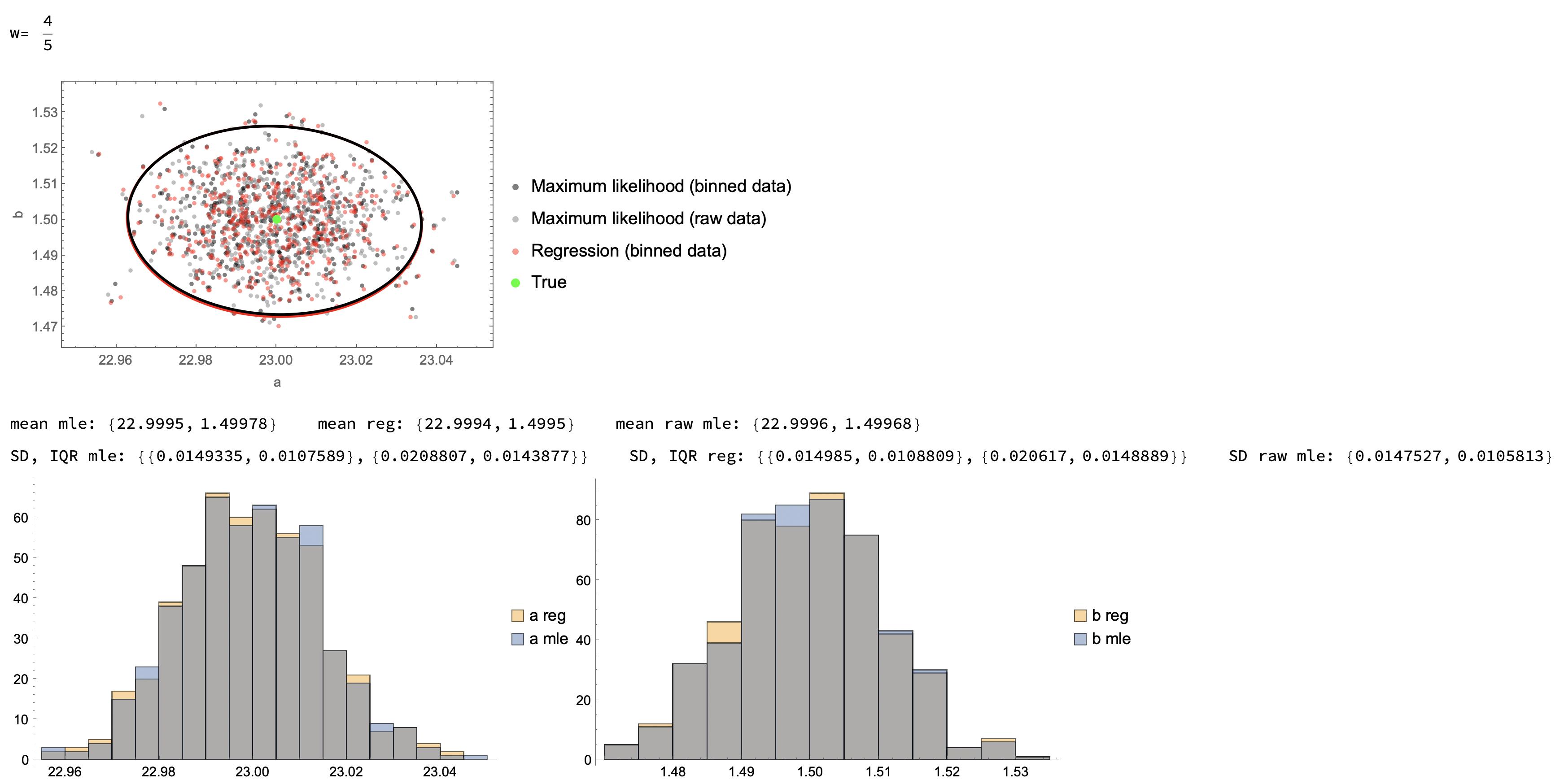
That is, if we have a Poisson process, and model it as such, the claim is that it will not differ from ML. To show this, with work in the chat link https://chat.stackexchange.com/rooms/137349/room-for-jimb-and-carl, the results of modelling are from simulation of a normal distribution with a sample size of 10000 performed 500 times. The synthetic mean "truth" value is 23 and the "true" SD is 3/2. Notice that the 95% tolerance ellipses largely superimpose, and the fits themselves are from fitting of bin width convolution of the normal distribution in both cases, MLE binned fitting, and regression binned fitting. To claim that regression is somehow inferior in quality to MLE, we would need to be careful as to which context we are speaking of, and in this case, there doesn't seem to be much of a difference for binned data.
To do ML, we can use @JimB's guess as to what the number of realizations are in each bin, duplicate that many samples in each bin at the bin location, and just use FindDistributionParameters, which is an ML procedure:
data3 = Rationalize[{{18.6, 1}, {18.84, 1}, {19.32, 1}, {19.56,
5}, {19.8, 3}, {20.04, 3}, {20.28, 11}, {20.52, 7}, {20.76,
4}, {21, 12}, {21.24, 13}, {21.48, 9}, {21.72, 22}, {21.96,
18}, {22.2, 37}, {22.44, 18}, {22.68, 22}, {22.92, 42}, {23.16,
20}, {23.4, 43}, {23.64, 33}, {23.88, 30}, {24.12, 36}, {24.36,
28}, {24.6, 32}, {24.84, 19}, {25.08, 18}, {25.32, 10}, {25.56,
9}, {25.8, 6}, {26.04, 10}, {26.28, 11}, {26.52, 4}, {26.76,
3}, {27, 2}, {27.24, 3}, {27.48, 4}, {27.72, 3}, {27.96,
1}, {28.92, 1}, {29.16, 1}}, 0];
datamess = Flatten[Table[data3[[i, 1]], {i, Length[data3]}, {j, 1, data3[[i, 2]]}]];

H1 = FindDistributionParameters[datamess, WeibullDistribution[a0, a1, a2], WorkingPrecision -> 30]
QQ1 = QuantilePlot[datamess, WeibullDistribution[a0, a1, a2] /. H1, PlotLabel -> "3 parm Weibull", ImageSize -> Medium];
H2 = FindDistributionParameters[datamess, WeibullDistribution[a0, a1], WorkingPrecision -> 30]
QQ2 = QuantilePlot[datamess, WeibullDistribution[a0, a1] /. H2, PlotLabel -> "2 parm Weibull", ImageSize -> Medium];
H3 = FindDistributionParameters[datamess, NormalDistribution[a0, a1], WorkingPrecision -> 30]
QQ3 = QuantilePlot[datamess, NormalDistribution[a0, a1] /. H3, PlotLabel -> "Normal", ImageSize -> Medium];
Print[QQ1, QQ2, QQ3]
Which gives us
 From the QQ plots, we can see the problem with just duplicating samples, we get a dotted step pattern $...\cdots$. Despite this, it is quite clear that the Normal distribution (see left tail) fits slightly better than the 3 parameter Weibull, which in turn fits much better than the 2 parameter Weibull.


