Return to Revisions

Here the problem was solved with a different perspective. You may find other solutions but what made this interesting to me was transforming one problem into another.

Here are the steps:

1. Create random points in 3d space
2. For each point, find points it covers
3. Build a graph out of these connections
4. Find a minimum set of points which can cover all the vertices by their neighborhood (aka cover all the pairs)

Assume we have a set of pairs:

SeedRandom[75];

pairs = RandomInteger[{0, 3}, {20, 3}];

n = Length[pairs];

pairs that have at least two similar axes will be associated for each pair, we can find them by:

Position[pairs, 
 Alternatives @@ 
  Table[ReplacePart[SOMEPAIR, i -> _], {i, 3}], {1}]

If we extend this code further, we could build an AdjacencyMatrix in which we want to select a minimum set of nodes that are never incident to the same edge (like FindIndependentVertexSet but in minimum terms):

graphRules = 
  DeleteDuplicatesBy[Sort]@
   Catenate@
    Table[Thread[
      index \[UndirectedEdge] 
       Catenate@
        Position[pairs, 
         Alternatives @@ 
          Table[ReplacePart[pairs[[index]], i -> _], {i, 
            3}], {1}]], {index, Length@pairs}];

adjacency = Unitize@AdjacencyMatrix[graphRules];

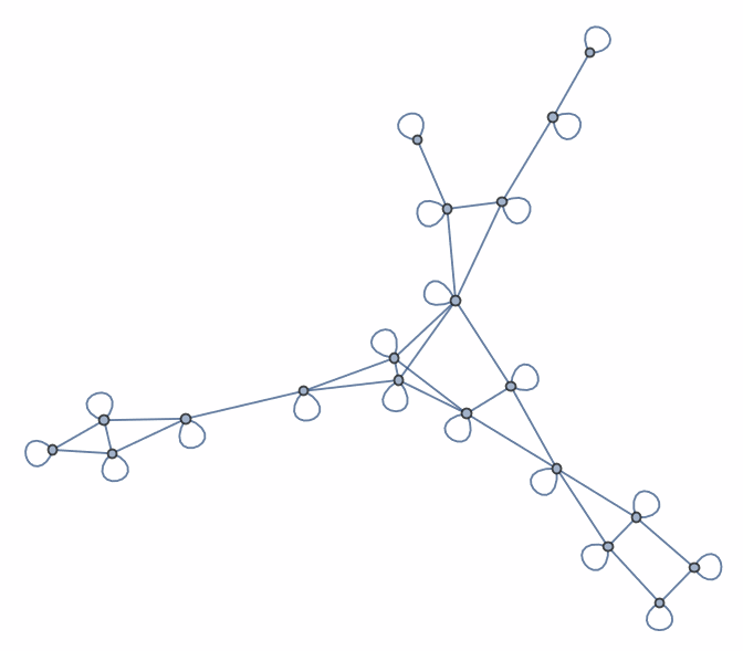
Showing the graph:

Graph[graphRules]

Now we find the vertex set:

result = LinearOptimization[
  ConstantArray[1,n],
 {Join[DiagonalMatrix@ConstantArray[1, n], adjacency], 
   Join[ConstantArray[0, n], ConstantArray[-1, n]]}, Integers]

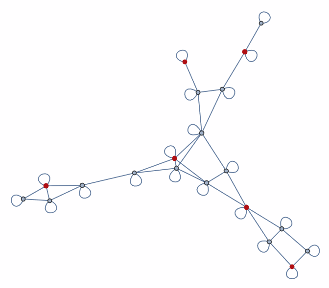
Highlighting the vertex set:

HighlightGraph[graphRules, 
 VertexList[graphRules][[Catenate@Position[result, 1]]]]

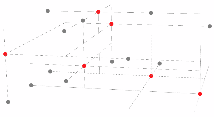
The red vertices in the above graph are the pairs you're looking for. Each vertex in the graph is either red or is in the neighborhood of a red vertex (aka is a chosen pair or is covered by a chosen pair). If we get the pairs:

pairs[[VertexList[graphRules][[Catenate@Position[result, 1]]]]]

(* Out: {{2, 3, 0}, {1, 2, 0}, {3, 0, 2}, {2, 1, 1}, {0, 1, 2}, {1, 1, 3}} *)

Visualizing the pairs:

Update 1

Since the above solution for large pairs like (Tuples[Range[0, 6, 1], 3]) takes quite a long time (mainly because of LinearOptimization), it could be faster in a static language. Here we'll discuss an alternative in Julia that is much faster than Mathematica in this particular case.

Requirement:

• Julia (is free and open-source, after installing follow Configure Julia for ExternalEvaluate)
• Package: JuMP.jl
• Package: HiGHS.jl

Now, start a Julia session:

juliaSession = 
 StartExternalSession[<|"System" -> "Julia", 
   "SessionProlog" -> "using JuMP, HiGHS"|>]

Define a function that accepts adjacency as input and returns the result:

juliaLinearOptimizer = ExternalFunction[juliaSession,
"function temp(data)
    
    n=size(data)[1];

    model = Model();
    set_optimizer(model,HiGHS.Optimizer);

    @variable(model,v[1:n],Bin)

    @objective(model,Min,sum(v[1:n]))

    for row in eachrow(data)
        @constraint(model,sum(v.*row)>=1)
    end

    optimize!(model)

    return round.(value.(v))
end"]

It solved the 6x6x6 in 40 seconds!

Floor @ Flatten @ juliaLinearOptimizer[Normal[adjacency]]

Don't forget to delete the object after you're done:

DeleteObject[juliaSession]

Comparison for 5x5x5