Return to Revisions

To make it easy, I'll use my EcoEvo package.

First time, you'll need to install it:

PacletInstall["EcoEvo", "Site" -> "http://raw.githubusercontent.com/cklausme/EcoEvo/master"]

Then, load the package to get started:

<<EcoEvo`

Both models are a little bit funny, in that total population size is conserved. Thus, model (i) is effectively one-dimensional and model (ii) is effectively two-dimensional.

Model (i): SI

SetModel[{
  Pop[pop] -> {
    Component[s] -> {Equation :> -β s i/n + γ i},
    Component[i] -> {Equation :> β s i/n - γ i}
  },
  Parameters :> {β > 0, γ > 0, n > 0}
}]

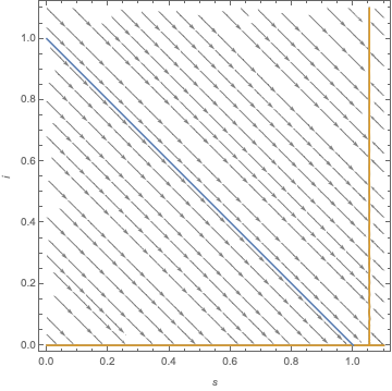
Let's go straight to the phase planes using PlotEcoPhasePlane, manually adding the total population constraint as a straight line. The subcritical case (disease-free equilibrium eq[[1]] is stable):

β = 0.95; γ = 1; n = 1;
Show[
 PlotEcoPhasePlane[{s, 0, 1.1}, {i, 0, 1.1}],
 Plot[n - s, {s, 0, n}]
]

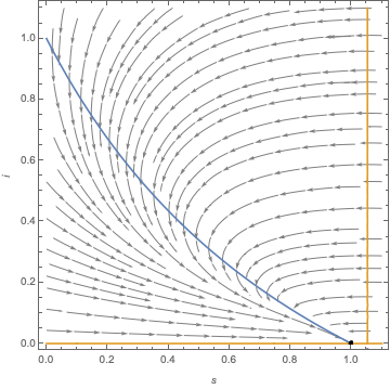
and the supercritical case (endemic equilibrium eq[[2]] is stable):

β = 4; γ = 1; n = 1;
Show[
 PlotEcoPhasePlane[{s, 0, 1}, {i, 0, 1}],
 Plot[n - s, {s, 0, n}]
]

Again, because of the total-population constraint, this is effectively a one-dimensional system with either two or one feasible (non-negative) equilibria.

Model (ii): SIR

Here we can get rid of the degeneracy by defining r := n - s - i, then work in the SI phase-plane.

r := n - s - i;
SetModel[{
  Pop[pop] -> {
    Component[s] -> {Equation :> -β s i/n + ξ r},
    Component[i] -> {Equation :> β s i/n - γ i}
  },
  Parameters :> {β > 0, γ > 0, ξ > 0}
}]

To verify your analytical results:

eq = SolveEcoEq[]

EcoEigenvalues[eq[[1]]]

EcoEigenvalues[eq[[2]]]

The eigenvalues of the non-trivial equilibrium are ugly, but we can check stability using Routh-Hurwitz criteria in EcoStableQ:

Simplify[EcoStableQ[eq[[2]]]]

On to the phase planes, to which I will include the equilibria (probably should automate this...).

Subcritical case:

β = 0.95; γ = 1; ξ = 1; n = 1;
eq = SolveEcoEq[];
Show[
 PlotEcoPhasePlane[{s, 0, 1.1}, {i, 0, 1.1}],
 RuleListPlot[eq, PlotMarkers -> EcoStableQ[eq]]
]

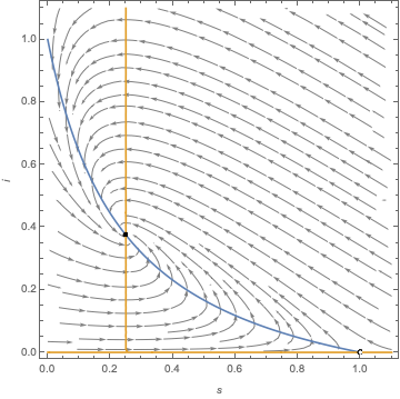
Supercritical case (stable focus, complex eigenvalues):

β = 4; γ = 1; ξ = 1; n = 1;
eq = SolveEcoEq[];
N[EcoEigenvalues[eq[[-1]]]]
Show[
 PlotEcoPhasePlane[{s, 0, 1.1}, {i, 0, 1.1}],
 RuleListPlot[eq, PlotMarkers -> EcoStableQ[eq]]
]
(* {-1.25 + 1.19896 I, -1.25 - 1.19896 I} *)

Supercritical case (stable node, real eigenvalues):

β = 4; γ = 1; ξ = 10; n = 1;
eq = SolveEcoEq[];
N[EcoEigenvalues[eq[[-1]]]]
Show[
 PlotEcoPhasePlane[{s, 0, 1.1}, {i, 0, 1.1}],
 RuleListPlot[eq, PlotMarkers -> EcoStableQ[eq]]
]
(* {-9.60337, -3.1239} *)