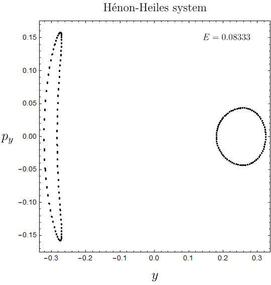
With the following code, you can plot the Poincaré sections of the Hénon-Heiles system:
With[{icv = {0, 0.36169437164930385`, 0.20100851639176504`, 0.029106357137938632`}},
solution = Reap[NDSolve[{x'[t] == px[t], px'[t] == -(x[t] + 2 x[t]* y[t]),
y'[t] == py[t], py'[t] == -(y[t] + x[t]^2 - y[t]^2),
x[0] == icv[[1]], px[0] == icv[[2]], y[0] == icv[[3]],
py[0] == icv[[4]]}, {x, px, y, py}, {t, 0, 1000},
MaxSteps -> \[Infinity],
Method -> {"EventLocator", "Event" -> x[t],
"EventAction" :> Sow[{y[t], py[t]}]}]];]
section = Part[solution, 2];
We load the MaTeX package for labels with LaTeX:
Needs["MaTeX`"];
Finally, we plot de Poincaré section:
ListPlot[section, PlotRange -> All, AspectRatio -> 1, PlotStyle -> Black,
Frame -> True, FrameStyle -> Black, Axes -> False, LabelStyle -> Directive[Black, Small],
FrameLabel -> {{MaTeX["p_{y}", Magnification -> 1.5], None},
{MaTeX["y", Magnification -> 1.5],
MaTeX["\\text{Hénon-Heiles system}", Magnification -> 1.3]}},
RotateLabel -> False, Epilog -> Inset[MaTeX["E=0.08333", Magnification -> 1],
{0.21, 0.15}, Automatic, 1], ImageSize -> Medium]
The Poincaré section:
You can use a For loop to compute with more initial conditions subject to the energy constraint of the Hénon-Heiles system. For more details, see my answer Poincaré Sections for spring pendulum

