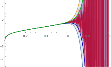
Here is another way to look at the OP's plot, which came to me after reading [Daniel Lichtblau's](http://mathematica.stackexchange.com/users/51/daniel-lichtblau) comment under the question.  His comment is worth emphasizing, which I think the following will show. ([Mr.Wizard](http://mathematica.stackexchange.com/users/121/mr-wizard) alludes to the issue in his remark on validity near the end of his answer.)

Let's say that machine precision is [binary64](http://en.wikipedia.org/wiki/Double-precision_floating-point_format), which has 53 bits of precision, and the maximum relative rounding error is `2^-53`.  Let's be a little fuzzy and say that the average error is roughly half that or `2^-54`.  The we can get almost exactly the envelope of the OP's plot as follows.  We can replace the coefficients with ones that are slightly larger and smaller (according with the maximum relative `error`); since `z >= 0`, the two resulting polynomials form estimates for the upper and lower bounds on `poly[z]`.  (I'll use a high working precision,  as in [Mr.Wizard's](http://mathematica.stackexchange.com/users/121/mr-wizard) answer, to compute the bounds precisely.)

    boundsPlot[error_, opts : OptionsPattern[Plot]] := With[{
        polyMin = poly[z] /. c_Real :> (1 - Sign[c] error) SetPrecision[c, Infinity],
        polyMax = poly[z] /. c_Real :> (1 + Sign[c] error) SetPrecision[c, Infinity]},
       Plot[{polyMin, polyMax}, {z, 0, 1}, WorkingPrecision -> 50, Filling -> {1 -> {2}}, opts]
       ];
    bounds = boundsPlot[2^-54, PlotStyle -> {Darker@Blue, Darker@Green}, PlotRange -> 5];
    absbounds = boundsPlot[2^-53, PlotRange -> 5];
    
    plotOP = Plot[poly[z], {z, 0, 1}, PlotStyle -> {AbsoluteThickness[0.7], Red}, PlotRange -> 5];
    
    Show[plotOP, absbounds, bounds]

![Mathematica graphics](https://i.sstatic.net/3qYu0.png)

A good way to think of floating-point numbers is that they represent an **interval** of real numbers.  At best a floating-point number is an approximation obtained by rounding the true value in an interval to the binary representative.  An average error of `2^-54` is about as precise as the coefficients could be if they are thought of as random variables uniformly distributed throughout each interval.  The `bounds` above show the range of likely possible values of `poly[z]`, although occasionally `poly[z]` exceeds `bounds`.

The upshot is this:   ***Under the hypothesis that the coefficients are known to `MachinePrecision`***, *the OP's original plot more accurately represents what is known about `poly[z]`, than the better-looking high-precision plot.*  The plot `bounds` seems to show the likely limits of the plot of the polynomial, under the same hypothesis (although calculating the probability is beyond me).  Similarly, the plot `absbounds` shows absolute bounds on the `poly[z]`.  Under the hypothesis, using `absbounds` or `bounds` seems the appropriate way to represent `poly[z]`.

If the error is greater than `2^-53`, say, because the coefficients are calculated from scientific measurements with less precision, then one can compute the corresponding bounds.