More complete solution added at the end.
Let's begin by assigning your object function to a function in order to make subsequent steps easier to see.
f[k_, r_, d_, s_] = (1/(2 (-1 + r)) (d^2 + 2 d k (-1 + r) - 2 d s +
   k (k + k (-3 + r) r + 2 r s)))/s^2;
Next, let's assume that there is a local minimum somewhere within the parameter space you have defined. If that is the case, then it must be true that the derivatives of this function with respect to k and r will be zero, and the second derivatives with respect to k and r will be negative. So:
Reduce[{D[f[k, r, d, s], k] == 0, D[f[k, r, d, s], r] == 0,
        D[f[k, r, d, s], {k, 2}] < 0, D[f[k, r, d, s], {r, 2}] < 0,
        k r < d, d <= k <= 1, 0 <= d <= 1, 2 d < s, r >= 0}, {k, r}]

(* False *)
This tells us that there are no conditions where there is a local minimum in the region. Therefore the true minimum must be on the boundary somewhere.
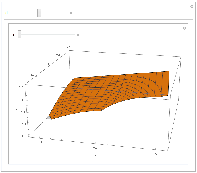
Let's see how to visualize this system. We are treating k and r as axes, and d and s as variable parameters. d takes on any values from 0 to 1, so we will have a Manipulate on the outside that lets us assign d within that range. s can take on any value greater than or equal to 2d, so we will have an inner Manipulate that allows you to set a value for s, bounded on the bottom by 2d, and we'll say 10 on the upper bound, but you can change that to whatever makes the most sense for you. Now we plot f[k,r,d,s] over the appropriate range of k and r. k can take on any value from d to 1, so that one is easy. r is a little harder because of the k r < d constraint, but in general r ranges from 0 to d/k. The maximum value of d/k comes at the minimum k (=d), so if we plot r from 0 to 1 we will have enough space. We can further restrict the domain to the correct region by using the RegionFunction option to Plot3D.
Manipulate[
  Manipulate[
    Plot3D[f[k, r, d, s], {k, d, 1}, {r, 0, 1},
      RegionFunction -> Function[{k, r, z}, (k r < d) && (1 > r >= 0)],
      AxesLabel -> {"k", "r", "f"}, ImageSize -> Large, PlotPoints -> 50,
      PlotRangePadding -> 0.1, WorkingPrecision -> 100],
    {s, 2 d, 10}],
  {{d, 0.5}, 0, 1}]
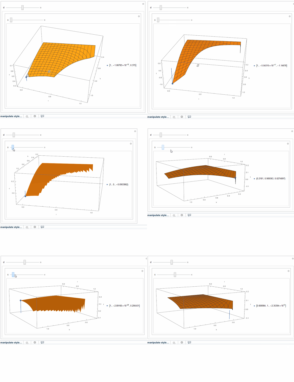
If you play with the resulting parameters, you can see why this is a difficult problem to solve analytically. Low values of d and s will give minima at k=1 and r=0. At higher values of s, the minimum shifts to k=1 and r=d. At higher values of d, the minimum visually looks to be anywhere along the k r = d boundary curve. And then there is the problem Mathematica has with handling the singularity near r=1 and k=d.
Given that the position of the minimum changes based on the parameters d and s, you may be better off specifying those values and then asking Mathematica to find the minimum:
Minimize[{f[k, r, 0.5, 2], k r < 0.5, r >= 0, 0.5 <= k <= 1}, {k, r}]

(* {-1.14162*10^14, {k -> 0.534188, r -> 1.}} *)
Here is a way to visualize the whole thing:
Manipulate[
  Manipulate[
    Show[Plot3D[f[k, r, d, s], {k, d, 1}, {r, 0, 1},
            RegionFunction -> Function[{k, r, z}, (k r < d) && (1 > r >= 0)],
            AxesLabel -> {"k", "r", "f"}, ImageSize -> Large,
            PlotPoints -> 50, PlotRangePadding -> 0.1,
            WorkingPrecision -> 100],
    ListPointPlot3D[{{k /. (#[[2]]), r /. (#[[2]]), #[[1]]}},
            Filling -> 0, FillingStyle -> Thick,
            PlotLegends -> {ToString[{k /. (#[[2]]), r /. (#[[2]]), #[[1]]},
                            StandardForm]}] &@
       Minimize[{f[k, r, d, s], k r < d, r >= 0, d <= k <= 1}, {k, r}]],
    {s, 2 d, 10}],
  {{d, 0.5}, 0, 1}]
All-in-all, this looks to be a problem that Minimize is not well-suited to.
More complete solution.
Having determined that the true minimum is on the boundary, we can look at the boundaries specifically. There are four lines/curves to examine:
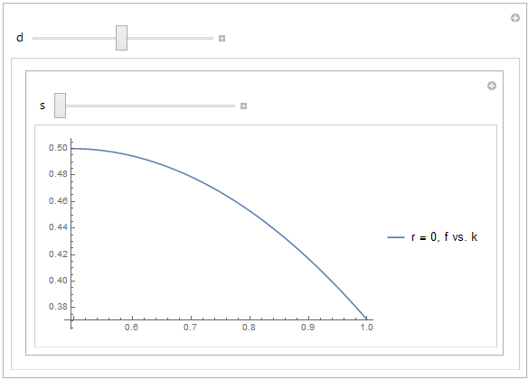
Line 1: r=0, k=d to 1
Manipulate[
  Manipulate[
    Plot[f[k, 0, d, s], {k, d, 1},
      PlotLegends -> {"r = 0, f vs. k"}],
  {s, 2 d, 10}],
{{d, 0.5}, 0, 1}]
Playing with the sliders will demonstrate to you that the minimum is always at k=1. Therefore Possibility 1 will be defined by {k,r}={1,0}, with a value of:
f[1, 0, d, s]

(* -((1 - 2 d + d^2 - 2 d s)/(2 s^2))  *)
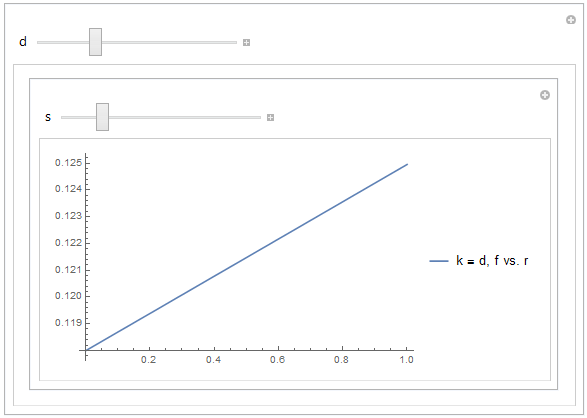
Line 2: k=d, r=0 to 1
Manipulate[
  Manipulate[
    Plot[f[d, r, d, s], {r, 0, 1},
      PlotLegends -> {"k = d, f vs. r"}],
    {s, 2 d, 10}],
  {{d, 0.5}, 0, 1}]
Playing with the sliders we can see that the minimum is always at r=0, which is the left-most point from line 1. And we already know that the right-most point from line 1 is always lower than the left-most point, so we have no new possibilities for a minimum here.
Line 3: k=1, r=0 to d
Manipulate[
  Manipulate[
    Plot[f[1, r, d, s], {r, 0, d},
      PlotLegends -> {"k = 1, f vs. r"}],
    {s, 2 d, 10}],
  {{d, 0.5}, 0, 1}]
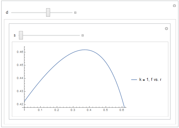
Playing with the slider here shows that the minimum could be either end of this line, depending on the values of d and s. The left-most point, {k,r}={1,0} is already Possibility 1. The right-most point is given by {k,r}={1,d} and has a value given by:
Simplify[f[1, d, d, s]]

(* (-1 + 4 d)/(2 s^2)  *)
We will call this Possibility 2.
Line 4: k=d to 1, while r=d/k at each point.
Manipulate[
  Manipulate[
    Plot[f[k, d/k, d, s], {k, d, 1},
      PlotLegends -> {"k = 1, r=d/k, f vs. k"}],
    {s, 2 d, 10}],
  {{d, 0.5}, 0, 1}]
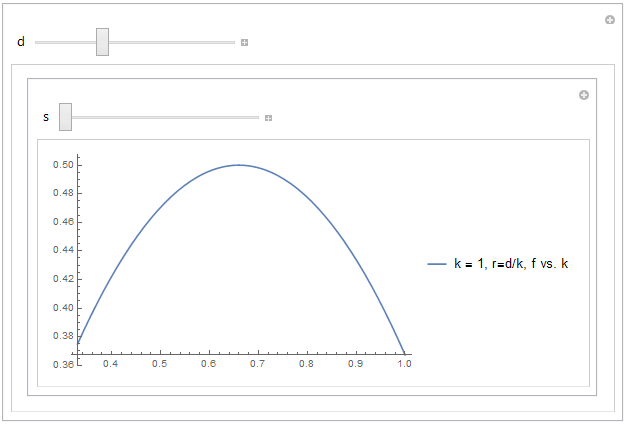
Again we find that the minimum along this line could be either end. The right-most possibility is Possibility 2, which we discussed above. The left-most point is a singularity, but we can take the limit, which we will call Possibility 3:
f[d, 1, d, s]

(* ComplexInfinity  *)

Limit[f[k, d/k, d, s], k -> d]

(*  (3 d^2)/(2 s^2)   *)
Summary
So there are three possible solutions:
- {k,r} = {1,0}, f = -((1 - 2 d + d^2 - 2 d s)/(2 s^2))
- {k,r} = {1,d}, f = (-1 + 4 d)/(2 s^2)
- {k,r} = {d,1}, f = (3 d^2)/(2 s^2)
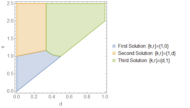
So when is each solution correct? Well, let's see:
one[d_,s_]=-((1 - 2 d + d^2 - 2 d s)/(2 s^2));
two[d_,s_]=(-1 + 4 d)/(2 s^2);
three[d_,s_]=(3 d^2)/(2 s^2);
The conditions under which the first solution is the true minimum are:
reg1=Reduce[{one[d, s] < two[d, s], one[d, s] < three[d, s], 0 <= d <= 1,
  2 d < s}, {d, s}]

(*  (0 < d <= 1/3 && 2 d < s < (2 + d)/2) || (1/3 < d < 1/2 &&
     2 d < s < (1 - 2 d + 4 d^2)/(2 d))   *)
The conditions under which the second solution is the true minimum are:
reg2=Reduce[{one[d, s] > two[d, s], two[d, s] < three[d, s], 0 <= d <= 1,
  2 d < s}, {d, s}]

(*  0 < d < 1/3 && s > (2 + d)/2  *)
And the conditions under which the third solution is the true minimum are:
reg3=Reduce[{one[d, s] > three[d, s], two[d, s] > three[d, s], 0 <= d <= 1,
  2 d < s}, {d, s}]

(*  (1/3 < d <= 1/2 && s > (1 - 2 d + 4 d^2)/(2 d)) ||
    (1/2 < d < 1 && s > 2 d)  *)
And we can visualize these conditions using a RegionPlot:
RegionPlot[{reg1, reg2, reg3}, {d, 0, 1}, {s, 0, 2.5},
  PlotLegends -> {"First Solution: {k,r}={1,0}",
                  "Second Solution: {k,r}={1,d}",
                  "Third Solution: {k,r}={d,1}"},
  FrameLabel -> {"d", "s"}, LabelStyle -> 16]
There's a moral here. As magnificent a package as Mathematica is, there is no substitute for breaking the problem down and thinking about it.

