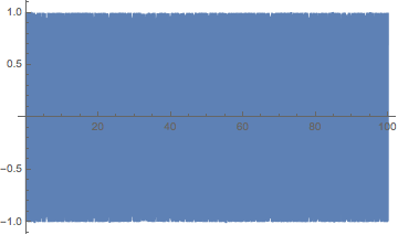
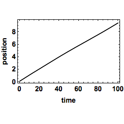
I think your dt=1 solution is the wrong one. The Cos[ν t] term is very rapidly varying with your parameter value of ν=105.:
Plot[Cos[ν t], {t, 0, tmax}, PlotPoints -> 200]

To get the right solution, I'd pick a time step much less than the period of the forcing.
Going out on a limb here, I'd guess that we could replace that rapidly varying Cos[ν t] term by its average of zero.
sme = ItoProcess[{\[DifferentialD]x[t] == y[t] \[DifferentialD]t,
  \[DifferentialD]y[t] == -\[Epsilon] Sin[x[t]] \[DifferentialD]w[t]},
  x[t], {{x, y}, {x0, y0}}, {t, 0},
  w \[Distributed] WienerProcess[drift, volatility]];
path = RandomFunction[sme, {0., tmax, 0.01}, 1]

Further speculation: the time average of -ϵ Sin[x[t]] \[DifferentialD]w[t] is zero, so the net effect of noise is zero. We might get some insights from the resulting ODE:
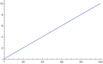
sol = NDSolve[{x'[t] == y[t], y'[t] == 0, x[0] == x0, y[0] == y0}, {x, y}, {t, 0, tmax}];
Plot[x[t] /. sol, {t, 0, tmax}]

I think for more interesting dynamics, you'll want to lower ν.
