Return to Revisions

[...] I am only interested in very fast numerical methods, no analytical results are needed.

[...] I have no idea how I can do it in Mathematica

The package AdaptiveNumericalLebesgueIntegration.m has Lebesgue integration strategy and rules implementations and it is discussed in detail in the blog post "Adaptive numerical Lebesgue integration by set measure estimates" and [3].

Using the profiling capabilities described in the referenced documents the speed of these Lebesgue integration algorithms can be evaluated for integrals of interest. Generally, for usual integrands, the algorithms are slower, but often require much less sampling points than, say, "AdaptiveMonteCarlo", which for expensively to evaluate integrands might produce results faster.

Lebesgue strategy and rules invocation examples

Here are examples of using the integration strategy and rules defined in the package:

Import["https://raw.githubusercontent.com/antononcube/MathematicaForPrediction/master/Misc/AdaptiveNumericalLebesgueIntegration.m"]

NIntegrate[Sqrt[x + y], {x, 0, 2}, {y, 0, 1}]
(* 2.38176 *)

NIntegrate[Sqrt[x + y], {x, 0, 2}, {y, 0, 1}, 
 Method -> {LebesgueIntegration, "Points" -> 2000, 
   "PointGenerator" -> "Sobol", "PointwiseMeasure" -> "VoronoiMesh"}, 
 PrecisionGoal -> 3]
(* 2.38236 *)

NIntegrate[Sqrt[x + y], {x, 0, 2}, {y, 0, 1}, 
 Method -> {LebesgueIntegrationRule, "Points" -> 6000, 
   "PointGenerator" -> "Sobol", "PointwiseMeasure" -> "VoronoiMesh", 
   "AxisSelector" -> {"MinVariance", "SubsampleFraction" -> 0.05}}, 
 PrecisionGoal -> 3]
(* 2.38095 *)

NIntegrate[Sqrt[x + y], {x, 0, 2}, {y, 0, 1}, 
 Method -> {GridLebesgueIntegrationRule, "Points" -> 2000, 
   "PointGenerator" -> Random, "GridSizes" -> 6, 
   "AxisSelector" -> Random}, 
 PrecisionGoal -> 3]
(* 2.37127 *)

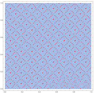
In the second integral above the strategy LebesgueIntegration uses the following Voronoi diagram to estimate the set measures:

For more details see the mentioned blog post.

Traces of Lebesgue integration process

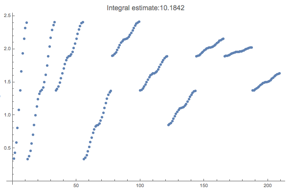
Here is an example that demonstrates the "dimension reduction" using the implemented Lebesgue integration strategy for a high dimensional (conventional) integral:

res = 
  Reap@NIntegrate[Sqrt[x + y + z], {x, 0, 2}, {y, 0, 1}, {z, 0, 3}, 
    Method -> {LebesgueIntegration, "Points" -> 12000, 
      "PointGenerator" -> Random, 
      "LebesgueIntegralVariableSymbol" -> f}, 
    EvaluationMonitor :> {Sow[f]}, PrecisionGoal -> 4, 
    MaxRecursion -> 7];
res = DeleteCases[res, f, \[Infinity]]

(* {10.1842, {{0.344945, 0.426233, 0.584845, 0.809906, 1.07998, 
   1.37175, 1.66352, ..., 1.50829, 
   1.51821, 1.53227, 1.54915, 1.56739, 1.58563, 1.6025, 1.61657, 
   1.62648, 1.63157}}} *)

 ListPlot[res[[2, 1]], 
  PlotLabel -> Style[Row[{"Integral estimate:", res[[1]]}], Larger]]

Compare with the result using the default NIntegrate algorithms:

NIntegrate[Sqrt[x + y + z], {x, 0, 2}, {y, 0, 1}, {z, 0, 3}]
(* 10.2016 *)

References

[1] B. L. Burrows, A new approach to numerical integration, 1. Inst. Math. Applics., 26(1980), 151-173.

[2] T. He, Dimensionality Reducing Expansion of Multivariate Integration, 2001, Birkhauser Boston. ISBN-13:978-1-4612-7414-8 .

[3] A. Antonov, Adaptive numerical Lebesgue integration by set measure estimates, (2016), MathematicaForPrediction project at GitHub.